利用ggpubr包进行R语言可视化

2016/08/12来源：R语言中文社区评论4,969

Hadley Wickham创建的可视化包ggplot2可以流畅地进行优美的可视化，但是如果要通过ggplot2定制一套图形，尤其是适用于杂志期刊等出版物的图形，对于那些没有深入了解ggplot2的人来说就有点困难了，ggplot2的部分语法是很晦涩的。为此Alboukadel Kassambara创建了基于ggplot2的可视化包ggpubr用于绘制符合出版物要求的图形。

安装及加载ggpubr包

安装方式有两种：

直接从CRAN安装：

install.packages("ggpubr")

从GitHub上安装最新版本：

if(!require(devtools)) 
install.packages("devtools") 
devtools::install_github("kassambara/ggpubr")

安装完之后直接加载就行：

library(ggpubr)

ggpubr可绘制图形

ggpubr可绘制大部分我们常用的图形，下面一一介绍。

分布图(Distribution)

#构建数据集set.seed(1234) 
 
df <- data.frame( sex=factor(rep(c("f", "M"), each=200)), weight=c(rnorm(200, 55), rnorm(200, 58))) 
head(df)
##   sex   weight
## 1  f   53.79293
## 2  f   55.27743
## 3  f   56.08444
## 4  f   52.65430
## 5  f   55.42912
## 6  f   55.50606

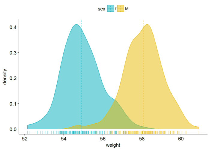
密度分布图以及边际地毯线并添加平均值线

ggdensity(df, x="weight", add = "mean", rug = TRUE, color = "sex", fill = "sex", palette = c("#00AFBB", "#E7B800"))

带有均值线和边际地毯线的直方图

gghistogram(df, x="weight", add = "mean", rug = TRUE, color = "sex", fill = "sex", palette = c("#00AFBB", "#E7B800"))

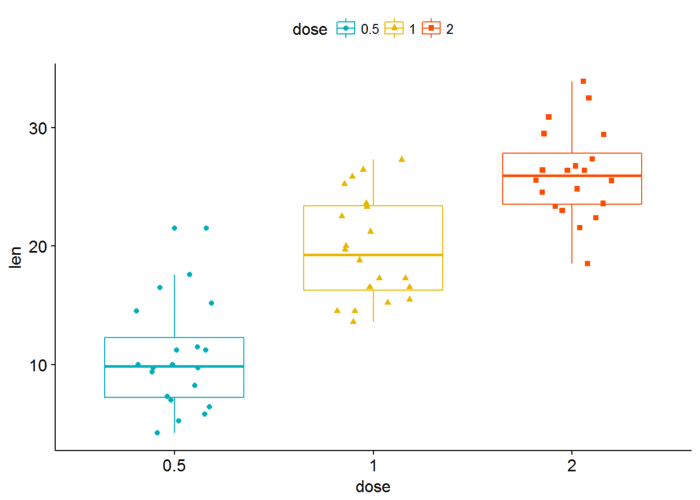
箱线图与小提琴图

#加载数据集ToothGrowth
 
data("ToothGrowth") 
df1 <- ToothGrowth head(df1)
##    len  supp  dose
## 1  4.2   VC    0.5
## 2  11.5  VC    0.5
## 3  7.3   VC    0.5
## 4  5.8   VC    0.5
## 5  6.4   VC    0.5
## 6  10.0  VC    0.5
p <- ggboxplot(df1, x="dose", y="len", color = "dose", palette = c("#00AFBB", "#E7B800", "#FC4E07"), add = "jitter", shape="dose")#增加了jitter点，点shape由dose映射p

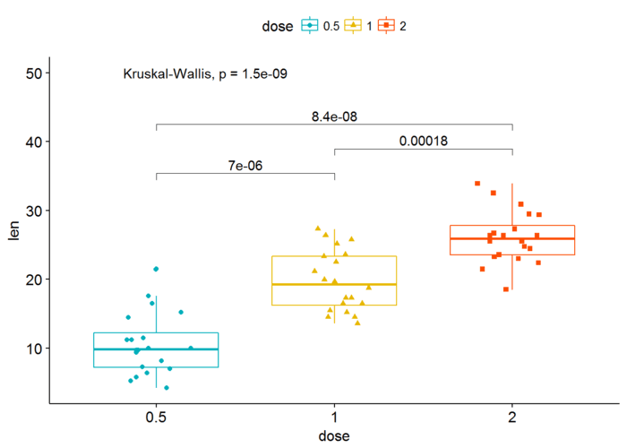
增加不同组间的p-value值，可以自定义需要标注的组间比较

my_comparisons <- list(c("0.5", "1"), c("1", "2"), c("0.5", "2")) p+stat_compare_means(comparisons = my_comparisons)+#不同组间的比较stat_compare_means(label.y=50)

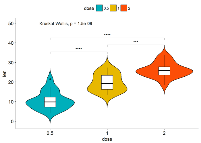
内有箱线图的小提琴图

ggviolin(df1, x="dose", y="len", fill = "dose", 
palette = c("#00AFBB", "#E7B800", "#FC4E07"), 
add = "boxplot", add.params = list(fill="white"))+ stat_compare_means(comparisons = my_comparisons, label ="p.signif") + stat_compare_means(label.y = 50)#label这里表示选择显著性标记（星号）

条形图

data("mtcars") 
 
df2 <- mtcars 
 
df2$cyl <- factor(df2$cyl)
 
df2$name <- rownames(df2)#添加一行name
 
head(df2[, c("name", "wt", "mpg", "cyl")])

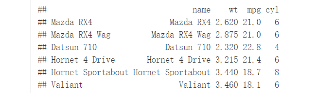
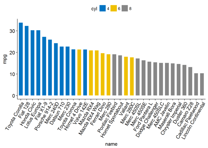
按从小到大顺序绘制条形图（不分组排序）

ggbarplot(df2, x="name", y="mpg", fill = "cyl", color = "white",
 
palette = "jco",#杂志jco的配色
 
sort.val = "desc",#下降排序
 
sort.by.groups=FALSE,#不按组排序
 
x.text.angle=60)

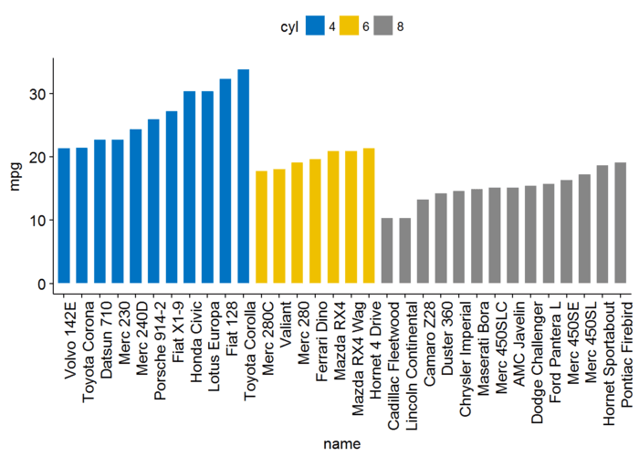
按组进行排序

ggbarplot(df2, x="name", y="mpg", fill = "cyl", color = "white",
 
palette = "jco",#杂志jco的配色
 
sort.val = "asc",#上升排序,区别于desc，具体看图演示
 
sort.by.groups=TRUE,#按组排序
 
x.text.angle=90)

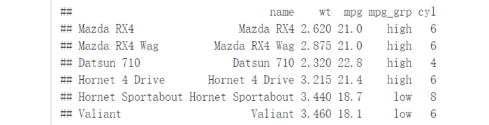
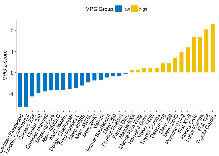
偏差图

偏差图展示了与参考值之间的偏差

df2$mpg_z <- (df2$mpg-mean(df2$mpg))/sd(df2$mpg) 
 
df2$mpg_grp <- factor(ifelse(df2$mpg_z<0, "low", "high"), levels = c("low", "high")) 
 
head(df2[, c("name", "wt", "mpg", "mpg_grp", "cyl")])

绘制排序过的条形图

ggbarplot(df2, x="name", y="mpg_z", fill = "mpg_grp", color = "white", 
 
palette = "jco", sort.val = "asc", sort.by.groups = FALSE, x.text.angle=60, ylab = "MPG z-score", xlab = FALSE, legend.title="MPG Group")

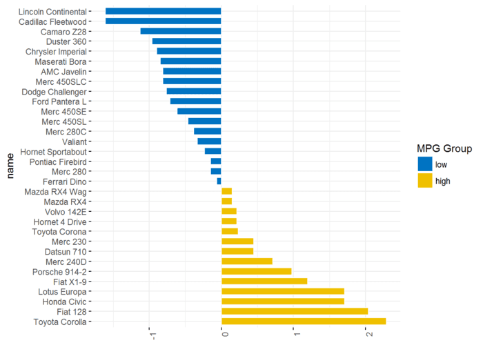
坐标轴变换

ggbarplot(df2, x="name", y="mpg_z", fill = "mpg_grp", color = "white", 
 
palette = "jco", sort.val = "desc", sort.by.groups = FALSE, 
 
x.text.angle=90, ylab = "MPG z-score", xlab = FALSE, 
 
legend.title="MPG Group", rotate=TRUE, ggtheme = theme_minimal())

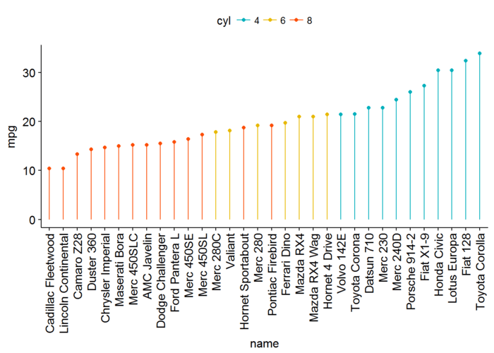
点图(Dot charts)

棒棒糖图(Lollipop chart)

棒棒图可以代替条形图展示数据

ggdotchart(df2, x="name", y="mpg", color = "cyl", 
 
palette = c("#00AFBB", "#E7B800", "#FC4E07"), sorting = "ascending", 
 
add = "segments", ggtheme = theme_pubr())

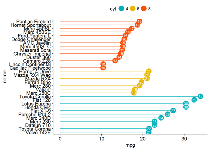
可以自设置各种参数

ggdotchart(df2, x="name", y="mpg", color = "cyl", 
 
palette = c("#00AFBB", "#E7B800", "#FC4E07"), sorting = "descending", 
 
add = "segments", rotate = TRUE, group = "cyl", dot.size = 6, 
 
label = round(df2$mpg), font.label = list(color="white", size=9, vjust=0.5), 
 
ggtheme = theme_pubr())

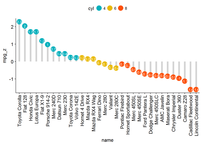
偏差图

ggdotchart(df2, x="name", y="mpg_z", color = "cyl", 
 
palette = c("#00AFBB", "#E7B800", "#FC4E07"), sorting = "descending", 
 
add = "segment", add.params = list(color="lightgray", size=2), 
 
group = "cyl", dot.size = 6, label = round(df2$mpg_z, 1), 
 
font.label = list(color="white", size=9, vjust=0.5),
 
ggtheme = theme_pubr())+ geom_line(yintercept=0, linetype=2, color="lightgray")

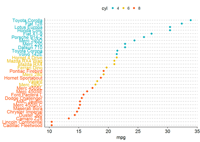
Cleveland点图

ggdotchart(df2, x="name", y="mpg", color = "cyl", 
 
palette = c("#00AFBB", "#E7B800", "#FC4E07"),
 
sorting = "descending", rotate = TRUE, dot.size = 2, y.text.col=TRUE, 
 
ggtheme = theme_pubr())+ theme_cleveland()

SessionInfo

sessionInfo()
 
## R version 3.4.0 (2017-04-21)
 
## Platform: x86_64-w64-mingw32/x64 (64-bit)
 
## Running under: Windows 8.1 x64 (build 9600)
 
##
 
## Matrix products: default
 
##
 
## locale:
 
## [1] LC_COLLATE=Chinese (Simplified)_China.936
 
## [2] LC_CTYPE=Chinese (Simplified)_China.936
 
## [3] LC_MONETARY=Chinese (Simplified)_China.936
 
## [4] LC_NUMERIC=C
 
## [5] LC_TIME=Chinese (Simplified)_China.936
 
##
 
## attached base packages:
 
## [1] stats graphics grDevices utils datasets methods base
 
##
 
## other attached packages:
 
## [1] ggpubr_0.1.3 magrittr_1.5 ggplot2_2.2.1
 
##
 
## loaded via a namespace (and not attached):
 
## [1] Rcpp_0.12.11 knitr_1.16 munsell_0.4.3 colorspace_1.3-2
 
## [5] R6_2.2.1 rlang_0.1.1 stringr_1.2.0 plyr_1.8.4
 
## [9] dplyr_0.5.0 tools_3.4.0 grid_3.4.0 gtable_0.2.0
 
## [13] DBI_0.6-1 htmltools_0.3.6 yaml_2.1.14 lazyeval_0.2.0
 
## [17] rprojroot_1.2 digest_0.6.12 assertthat_0.2.0 tibble_1.3.3
 
## [21] ggsignif_0.2.0 ggsci_2.4 purrr_0.2.2.2 evaluate_0.10
 
## [25] rmarkdown_1.5 labeling_0.3 stringi_1.1.5 compiler_3.4.0
 
## [29] scales_0.4.1 backports_1.1.0

发表评论