

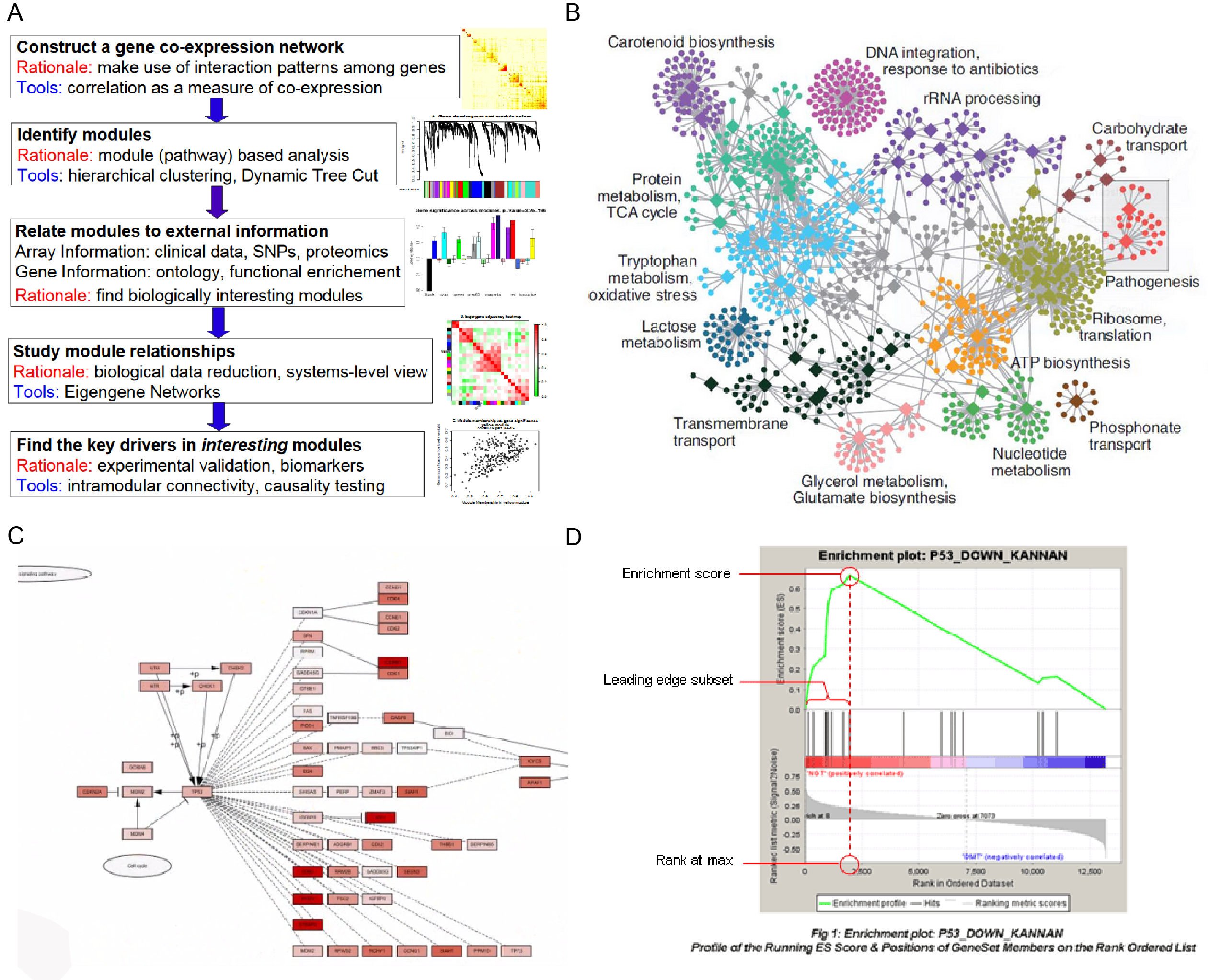
WGCNA基本概念
加权基因共表达网络分析 (WGCNA, Weighted correlation network analysis)是用来描述不同样品之间基因关联模式的系统生物学方法,可以用来鉴定高度协同变化的基因集, 并根据基因集的内连性和基因集与表型之间的关联鉴定候补生物标记基因或治疗靶点。
相比于只关注差异表达的基因,WGCNA利用数千或近万个变化最大的基因或全部基因的信息识别感兴趣的基因集,并与表型进行显著性关联分析。一是充分利用了信息,二是把数千个基因与表型的关联转换为数个基因集与表型的关联,免去了多重假设检验校正的问题。
理解WGCNA,需要先理解下面几个术语和它们在WGCNA中的定义。
- 共表达网络:定义为加权基因网络。点代表基因,边代表基因表达相关性。加权是指对相关性值进行冥次运算 (冥次的值也就是软阈值 (power, pickSoftThreshold这个函数所做的就是确定合适的power))。无向网络的边属性计算方式为
abs(cor(genex, geney)) ^ power;有向网络的边属性计算方式为(1+cor(genex, geney)/2) ^ power; sign hybrid的边属性计算方式为cor(genex, geney)^power if cor>0 else 0。这种处理方式强化了强相关,弱化了弱相关或负相关,使得相关性数值更符合无标度网络特征,更具有生物意义。如果没有合适的power,一般是由于部分样品与其它样品因为某种原因差别太大导致的,可根据具体问题移除部分样品或查看后面的经验值。 - Module(模块):高度內连的基因集。在无向网络中,模块内是高度相关的基因。在有向网络中,模块内是高度正相关的基因。把基因聚类成模块后,可以对每个模块进行三个层次的分析:
1. 功能富集分析查看其功能特征是否与研究目的相符;2. 模块与性状进行关联分析,找出与关注性状相关度最高的模块;3. 模块与样本进行关联分析,找到样品特异高表达的模块。 - Connectivity (连接度):类似于网络中 “度” (degree)的概念。每个基因的连接度是与其相连的基因的
边属性之和。 - Module eigengene E: 给定模型的第一主成分,代表整个模型的基因表达谱。这个是个很巧妙的梳理,我们之前讲过PCA分析的降维作用,之前主要是拿来做可视化,现在用到这个地方,很好的用一个向量代替了一个矩阵,方便后期计算。(降维除了PCA,还可以看看tSNE)
- Intramodular connectivity: 给定基因与给定模型内其他基因的关联度,判断基因所属关系。
- Module membership: 给定基因表达谱与给定模型的eigengene的相关性。
- Hub gene: 关键基因 (连接度最多或连接多个模块的基因)。
- Adjacency matrix (邻接矩阵):基因和基因之间的加权相关性值构成的矩阵。
- TOM (Topological overlap matrix):把邻接矩阵转换为拓扑重叠矩阵,以降低噪音和假相关,获得的新距离矩阵,这个信息可拿来构建网络或绘制TOM图。
基本分析流程
- 构建基因共表达网络:使用加权的表达相关性。
- 识别基因集:基于加权相关性,进行层级聚类分析,并根据设定标准切分聚类结果,获得不同的基因模块,用聚类树的分枝和不同颜色表示。
- 如果有表型信息,计算基因模块与表型的相关性,鉴定性状相关的模块。
- 研究模型之间的关系,从系统层面查看不同模型的互作网络。
- 从关键模型中选择感兴趣的驱动基因,或根据模型中已知基因的功能推测未知基因的功能。
- 导出TOM矩阵,绘制相关性图。
WGCNA包实战
R包WGCNA是用于计算各种加权关联分析的功能集合,可用于网络构建,基因筛选,基因簇鉴定,拓扑特征计算,数据模拟和可视化等。
输入数据和参数选择
- WGCNA本质是基于相关系数的网络分析方法,适用于多样品数据模式,一般要求样本数多于15个。样本数多于20时效果更好,样本越多,结果越稳定。
- 基因表达矩阵: 常规表达矩阵即可,即基因在行,样品在列,进入分析前做一个转置。RPKM、FPKM或其它标准化方法影响不大,推荐使用Deseq2的
varianceStabilizingTransformation或log2(x+1)对标准化后的数据做个转换。如果数据来自不同的批次,需要先移除批次效应 (记得上次转录组培训课讲过如何操作)。如果数据存在系统偏移,需要做下quantile normalization。 - 性状矩阵:用于关联分析的性状必须是数值型特征 (如下面示例中的
Height,Weight,Diameter)。如果是区域或分类变量,需要转换为0-1矩阵的形式(1表示属于此组或有此属性,0表示不属于此组或无此属性,如样品分组信息WT, KO, OE)。- ID WT KO OE Height Weight Diameter
- samp1 1 0 0 1 2 3
- samp2 1 0 0 2 4 6
- samp3 0 1 0 10 20 50
- samp4 0 1 0 15 30 80
- samp5 0 0 1 NA 9 8
- samp6 0 0 1 4 8 7
- 推荐使用
Signed network和Robust correlation (bicor)。(这个根据自己的需要,看看上面写的每个网络怎么计算的,更知道怎么选择) - 无向网络在power小于
15或有向网络power小于30内,没有一个power值可以使无标度网络图谱结构R^2达到0.8或平均连接度降到100以下,可能是由于部分样品与其他样品差别太大造成的。这可能由批次效应、样品异质性或实验条件对表达影响太大等造成, 可以通过绘制样品聚类查看分组信息、关联批次信息、处理信息和有无异常样品 (可以使用之前讲过的热图简化,增加行或列属性)。如果这确实是由有意义的生物变化引起的,也可以使用后面程序中的经验power值。
安装WGCNA
WGCNA依赖的包比较多,bioconductor上的包需要自己安装,cran上依赖的包可以自动安装。通常在R中运行下面4条语句就可以完成WGCNA的安装。
建议在编译安装R时增加--with-blas --with-lapack提高矩阵运算的速度,具体见R和Rstudio安装。
- #source("https://bioconductor.org/biocLite.R")
- #biocLite(c("AnnotationDbi", "impute","GO.db", "preprocessCore"))
- #site="https://mirrors.tuna.tsinghua.edu.cn/CRAN"
- #install.packages(c("WGCNA", "stringr", "reshape2"), repos=site)
WGCNA实战
实战采用的是官方提供的清理后的矩阵,原矩阵信息太多,容易给人误导,后台回复 WGCNA 获取数据。
数据读入
- library(WGCNA)
- ## Loading required package: dynamicTreeCut
- ## Loading required package: fastcluster
- ##
- ## Attaching package: 'fastcluster'
- ## The following object is masked from 'package:stats':
- ##
- ## hclust
- ## ==========================================================================
- ## *
- ## * Package WGCNA 1.63 loaded.
- ## *
- ## * Important note: It appears that your system supports multi-threading,
- ## * but it is not enabled within WGCNA in R.
- ## * To allow multi-threading within WGCNA with all available cores, use
- ## *
- ## * allowWGCNAThreads()
- ## *
- ## * within R. Use disableWGCNAThreads() to disable threading if necessary.
- ## * Alternatively, set the following environment variable on your system:
- ## *
- ## * ALLOW_WGCNA_THREADS=<number_of_processors>
- ## *
- ## * for example
- ## *
- ## * ALLOW_WGCNA_THREADS=48
- ## *
- ## * To set the environment variable in linux bash shell, type
- ## *
- ## * export ALLOW_WGCNA_THREADS=48
- ## *
- ## * before running R. Other operating systems or shells will
- ## * have a similar command to achieve the same aim.
- ## *
- ## ==========================================================================
- ##
- ## Attaching package: 'WGCNA'
- ## The following object is masked from 'package:stats':
- ##
- ## cor
- library(reshape2)
- library(stringr)
- #
- options(stringsAsFactors = FALSE)
- # 打开多线程
- enableWGCNAThreads()
- ## Allowing parallel execution with up to 47 working processes.
- # 常规表达矩阵,log2转换后或
- # Deseq2的varianceStabilizingTransformation转换的数据
- # 如果有批次效应,需要事先移除,可使用removeBatchEffect
- # 如果有系统偏移(可用boxplot查看基因表达分布是否一致),
- # 需要quantile normalization
- exprMat <- "WGCNA/LiverFemaleClean.txt"
- # 官方推荐 "signed" 或 "signed hybrid"
- # 为与原文档一致,故未修改
- type = "unsigned"
- # 相关性计算
- # 官方推荐 biweight mid-correlation & bicor
- # corType: pearson or bicor
- # 为与原文档一致,故未修改
- corType = "pearson"
- corFnc = ifelse(corType=="pearson", cor, bicor)
- # 对二元变量,如样本性状信息计算相关性时,
- # 或基因表达严重依赖于疾病状态时,需设置下面参数
- maxPOutliers = ifelse(corType=="pearson",1,0.05)
- # 关联样品性状的二元变量时,设置
- robustY = ifelse(corType=="pearson",T,F)
- ##导入数据##
- dataExpr <- read.table(exprMat, sep='\t', row.names=1, header=T,
- quote="", comment="", check.names=F)
- dim(dataExpr)
- ## [1] 3600 134
- head(dataExpr)[,1:8]
- ## F2_2 F2_3 F2_14 F2_15 F2_19 F2_20
- ## MMT00000044 -0.01810 0.0642 6.44e-05 -0.05800 0.04830 -0.15197410
- ## MMT00000046 -0.07730 -0.0297 1.12e-01 -0.05890 0.04430 -0.09380000
- ## MMT00000051 -0.02260 0.0617 -1.29e-01 0.08710 -0.11500 -0.06502607
- ## MMT00000076 -0.00924 -0.1450 2.87e-02 -0.04390 0.00425 -0.23610000
- ## MMT00000080 -0.04870 0.0582 -4.83e-02 -0.03710 0.02510 0.08504274
- ## MMT00000102 0.17600 -0.1890 -6.50e-02 -0.00846 -0.00574 -0.01807182
- ## F2_23 F2_24
- ## MMT00000044 -0.00129 -0.23600
- ## MMT00000046 0.09340 0.02690
- ## MMT00000051 0.00249 -0.10200
- ## MMT00000076 -0.06900 0.01440
- ## MMT00000080 0.04450 0.00167
- ## MMT00000102 -0.12500 -0.06820
数据筛选
- ## 筛选中位绝对偏差前75%的基因,至少MAD大于0.01
- ## 筛选后会降低运算量,也会失去部分信息
- ## 也可不做筛选,使MAD大于0即可
- m.mad <- apply(dataExpr,1,mad)
- dataExprVar <- dataExpr[which(m.mad >
- max(quantile(m.mad, probs=seq(0, 1, 0.25))[2],0.01)),]
- ## 转换为样品在行,基因在列的矩阵
- dataExpr <- as.data.frame(t(dataExprVar))
- ## 检测缺失值
- gsg = goodSamplesGenes(dataExpr, verbose = 3)
- ## Flagging genes and samples with too many missing values...
- ## ..step 1
- if (!gsg$allOK){
- # Optionally, print the gene and sample names that were removed:
- if (sum(!gsg$goodGenes)>0)
- printFlush(paste("Removing genes:",
- paste(names(dataExpr)[!gsg$goodGenes], collapse = ",")));
- if (sum(!gsg$goodSamples)>0)
- printFlush(paste("Removing samples:",
- paste(rownames(dataExpr)[!gsg$goodSamples], collapse = ",")));
- # Remove the offending genes and samples from the data:
- dataExpr = dataExpr[gsg$goodSamples, gsg$goodGenes]
- }
- nGenes = ncol(dataExpr)
- nSamples = nrow(dataExpr)
- dim(dataExpr)
- ## [1] 134 2697
- head(dataExpr)[,1:8]
- ## MMT00000051 MMT00000080 MMT00000102 MMT00000149 MMT00000159
- ## F2_2 -0.02260000 -0.04870000 0.17600000 0.07680000 -0.14800000
- ## F2_3 0.06170000 0.05820000 -0.18900000 0.18600000 0.17700000
- ## F2_14 -0.12900000 -0.04830000 -0.06500000 0.21400000 -0.13200000
- ## F2_15 0.08710000 -0.03710000 -0.00846000 0.12000000 0.10700000
- ## F2_19 -0.11500000 0.02510000 -0.00574000 0.02100000 -0.11900000
- ## F2_20 -0.06502607 0.08504274 -0.01807182 0.06222751 -0.05497686
- ## MMT00000207 MMT00000212 MMT00000241
- ## F2_2 0.06870000 0.06090000 -0.01770000
- ## F2_3 0.10100000 0.05570000 -0.03690000
- ## F2_14 0.10900000 0.19100000 -0.15700000
- ## F2_15 -0.00858000 -0.12100000 0.06290000
- ## F2_19 0.10500000 0.05410000 -0.17300000
- ## F2_20 -0.02441415 0.06343181 0.06627665
软阈值筛选
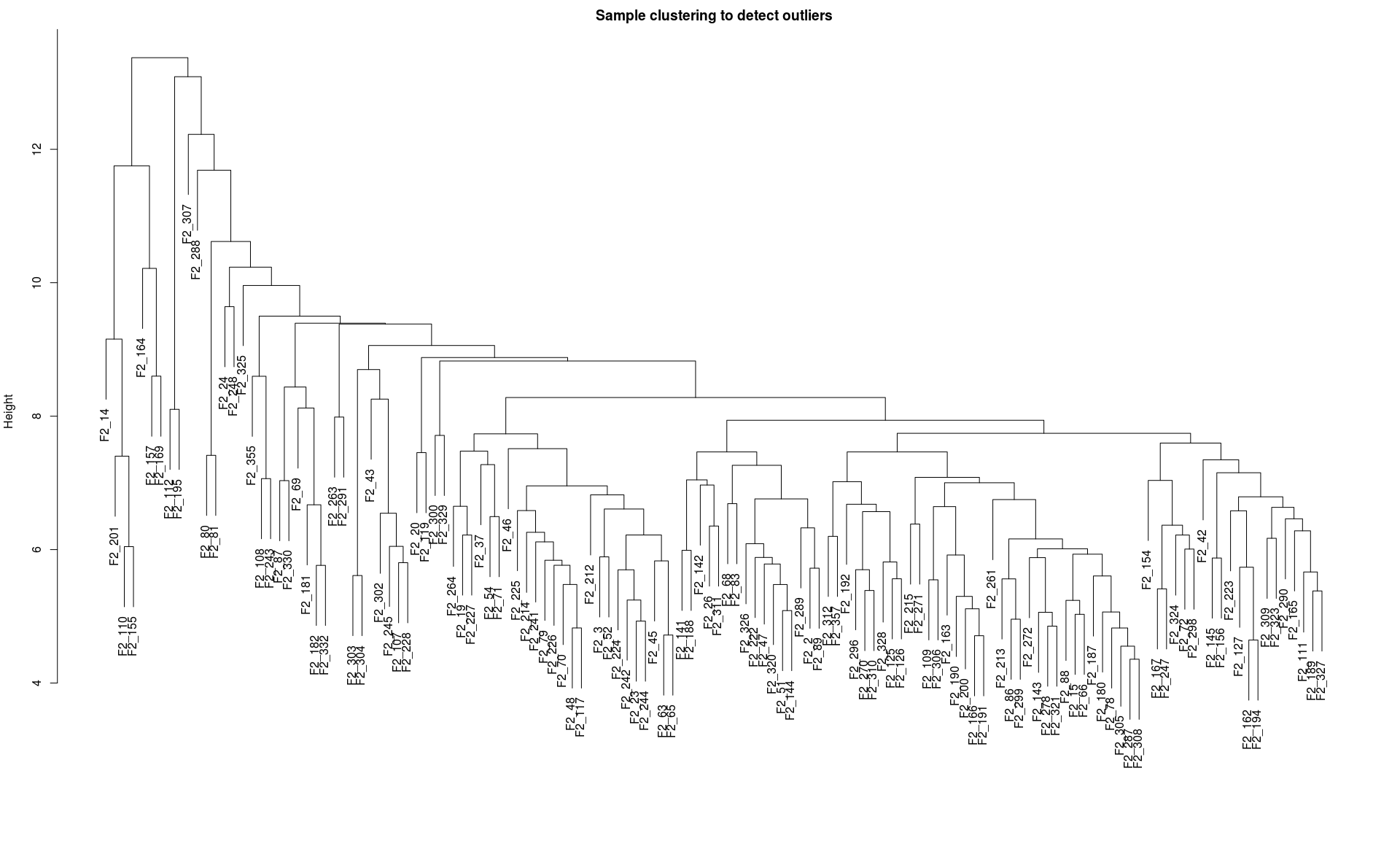
- ## 查看是否有离群样品
- sampleTree = hclust(dist(dataExpr), method = "average")
- plot(sampleTree, main = "Sample clustering to detect outliers", sub="", xlab="")
软阈值的筛选原则是使构建的网络更符合无标度网络特征。
- powers = c(c(1:10), seq(from = 12, to=30, by=2))
- sft = pickSoftThreshold(dataExpr, powerVector=powers,
- networkType=type, verbose=5)
- ## pickSoftThreshold: will use block size 2697.
- ## pickSoftThreshold: calculating connectivity for given powers...
- ## ..working on genes 1 through 2697 of 2697
- ## Power SFT.R.sq slope truncated.R.sq mean.k. median.k. max.k.
- ## 1 1 0.1370 0.825 0.412 587.000 5.95e+02 922.0
- ## 2 2 0.0416 -0.332 0.630 206.000 2.02e+02 443.0
- ## 3 3 0.2280 -0.747 0.920 91.500 8.43e+01 247.0
- ## 4 4 0.3910 -1.120 0.908 47.400 4.02e+01 154.0
- ## 5 5 0.7320 -1.230 0.958 27.400 2.14e+01 102.0
- ## 6 6 0.8810 -1.490 0.916 17.200 1.22e+01 83.7
- ## 7 7 0.8940 -1.640 0.869 11.600 7.29e+00 75.4
- ## 8 8 0.8620 -1.660 0.827 8.250 4.56e+00 69.2
- ## 9 9 0.8200 -1.600 0.810 6.160 2.97e+00 64.2
- ## 10 10 0.8390 -1.560 0.855 4.780 2.01e+00 60.1
- ## 11 12 0.8020 -1.410 0.866 3.160 9.61e-01 53.2
- ## 12 14 0.8470 -1.340 0.909 2.280 4.84e-01 47.7
- ## 13 16 0.8850 -1.250 0.932 1.750 2.64e-01 43.1
- ## 14 18 0.8830 -1.210 0.922 1.400 1.46e-01 39.1
- ## 15 20 0.9110 -1.180 0.926 1.150 8.35e-02 35.6
- ## 16 22 0.9160 -1.140 0.927 0.968 5.02e-02 32.6
- ## 17 24 0.9520 -1.120 0.961 0.828 2.89e-02 29.9
- ## 18 26 0.9520 -1.120 0.944 0.716 1.77e-02 27.5
- ## 19 28 0.9380 -1.120 0.922 0.626 1.08e-02 25.4
- ## 20 30 0.9620 -1.110 0.951 0.551 6.49e-03 23.5
- par(mfrow = c(1,2))
- cex1 = 0.9
- # 横轴是Soft threshold (power),纵轴是无标度网络的评估参数,数值越高,
- # 网络越符合无标度特征 (non-scale)
- plot(sft$fitIndices[,1], -sign(sft$fitIndices[,3])*sft$fitIndices[,2],
- xlab="Soft Threshold (power)",
- ylab="Scale Free Topology Model Fit,signed R^2",type="n",
- main = paste("Scale independence"))
- text(sft$fitIndices[,1], -sign(sft$fitIndices[,3])*sft$fitIndices[,2],
- labels=powers,cex=cex1,col="red")
- # 筛选标准。R-square=0.85
- abline(h=0.85,col="red")
- # Soft threshold与平均连通性
- plot(sft$fitIndices[,1], sft$fitIndices[,5],
- xlab="Soft Threshold (power)",ylab="Mean Connectivity", type="n",
- main = paste("Mean connectivity"))
- text(sft$fitIndices[,1], sft$fitIndices[,5], labels=powers,
- cex=cex1, col="red")
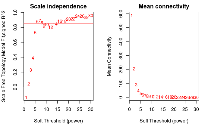
- power = sft$powerEstimate
- power
- ## [1] 6
经验power (无满足条件的power时选用)
- # 无向网络在power小于15或有向网络power小于30内,没有一个power值可以使
- # 无标度网络图谱结构R^2达到0.8,平均连接度较高如在100以上,可能是由于
- # 部分样品与其他样品差别太大。这可能由批次效应、样品异质性或实验条件对
- # 表达影响太大等造成。可以通过绘制样品聚类查看分组信息和有无异常样品。
- # 如果这确实是由有意义的生物变化引起的,也可以使用下面的经验power值。
- if (is.na(power)){
- power = ifelse(nSamples<20, ifelse(type == "unsigned", 9, 18),
- ifelse(nSamples<30, ifelse(type == "unsigned", 8, 16),
- ifelse(nSamples<40, ifelse(type == "unsigned", 7, 14),
- ifelse(type == "unsigned", 6, 12))
- )
- )
- }
网络构建
- ##一步法网络构建:One-step network construction and module detection##
- # power: 上一步计算的软阈值
- # maxBlockSize: 计算机能处理的最大模块的基因数量 (默认5000);
- # 4G内存电脑可处理8000-10000个,16G内存电脑可以处理2万个,32G内存电脑可
- # 以处理3万个
- # 计算资源允许的情况下最好放在一个block里面。
- # corType: pearson or bicor
- # numericLabels: 返回数字而不是颜色作为模块的名字,后面可以再转换为颜色
- # saveTOMs:最耗费时间的计算,存储起来,供后续使用
- # mergeCutHeight: 合并模块的阈值,越大模块越少
- net = blockwiseModules(dataExpr, power = power, maxBlockSize = nGenes,
- TOMType = type, minModuleSize = 30,
- reassignThreshold = 0, mergeCutHeight = 0.25,
- numericLabels = TRUE, pamRespectsDendro = FALSE,
- saveTOMs=TRUE, corType = corType,
- maxPOutliers=maxPOutliers, loadTOMs=TRUE,
- saveTOMFileBase = paste0(exprMat, ".tom"),
- verbose = 3)
- ## Calculating module eigengenes block-wise from all genes
- ## Flagging genes and samples with too many missing values...
- ## ..step 1
- ## ..Working on block 1 .
- ## TOM calculation: adjacency..
- ## ..will use 47 parallel threads.
- ## Fraction of slow calculations: 0.000000
- ## ..connectivity..
- ## ..matrix multiplication (system BLAS)..
- ## ..normalization..
- ## ..done.
- ## ..saving TOM for block 1 into file WGCNA/LiverFemaleClean.txt.tom-block.1.RData
- ## ....clustering..
- ## ....detecting modules..
- ## ....calculating module eigengenes..
- ## ....checking kME in modules..
- ## ..removing 3 genes from module 1 because their KME is too low.
- ## ..removing 5 genes from module 12 because their KME is too low.
- ## ..removing 1 genes from module 14 because their KME is too low.
- ## ..merging modules that are too close..
- ## mergeCloseModules: Merging modules whose distance is less than 0.25
- ## Calculating new MEs...
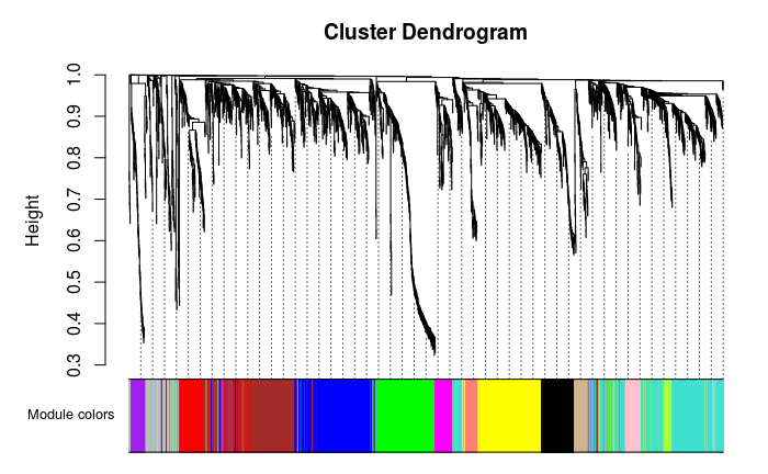
- # 根据模块中基因数目的多少,降序排列,依次编号为 `1-最大模块数`。
- # **0 (grey)**表示**未**分入任何模块的基因。
- table(net$colors)
- ##
- ## 0 1 2 3 4 5 6 7 8 9 10 11 12 13
- ## 135 472 356 333 307 303 177 158 102 94 69 66 63 62
层级聚类树展示各个模块
- ## 灰色的为**未分类**到模块的基因。
- # Convert labels to colors for plotting
- moduleLabels = net$colors
- moduleColors = labels2colors(moduleLabels)
- # Plot the dendrogram and the module colors underneath
- # 如果对结果不满意,还可以recutBlockwiseTrees,节省计算时间
- plotDendroAndColors(net$dendrograms[[1]], moduleColors[net$blockGenes[[1]]],
- "Module colors",
- dendroLabels = FALSE, hang = 0.03,
- addGuide = TRUE, guideHang = 0.05)
绘制模块之间相关性图
- # module eigengene, 可以绘制线图,作为每个模块的基因表达趋势的展示
- MEs = net$MEs
- ### 不需要重新计算,改下列名字就好
- ### 官方教程是重新计算的,起始可以不用这么麻烦
- MEs_col = MEs
- colnames(MEs_col) = paste0("ME", labels2colors(
- as.numeric(str_replace_all(colnames(MEs),"ME",""))))
- MEs_col = orderMEs(MEs_col)
- # 根据基因间表达量进行聚类所得到的各模块间的相关性图
- # marDendro/marHeatmap 设置下、左、上、右的边距
- plotEigengeneNetworks(MEs_col, "Eigengene adjacency heatmap",
- marDendro = c(3,3,2,4),
- marHeatmap = c(3,4,2,2), plotDendrograms = T,
- xLabelsAngle = 90)
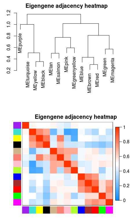
- ## 如果有表型数据,也可以跟ME数据放一起,一起出图
- #MEs_colpheno = orderMEs(cbind(MEs_col, traitData))
- #plotEigengeneNetworks(MEs_colpheno, "Eigengene adjacency heatmap",
- # marDendro = c(3,3,2,4),
- # marHeatmap = c(3,4,2,2), plotDendrograms = T,
- # xLabelsAngle = 90)
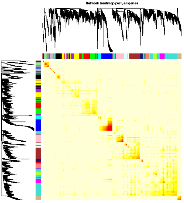
可视化基因网络 (TOM plot)
- # 如果采用分步计算,或设置的blocksize>=总基因数,直接load计算好的TOM结果
- # 否则需要再计算一遍,比较耗费时间
- # TOM = TOMsimilarityFromExpr(dataExpr, power=power, corType=corType, networkType=type)
- load(net$TOMFiles[1], verbose=T)
- ## Loading objects:
- ## TOM
- TOM <- as.matrix(TOM)
- dissTOM = 1-TOM
- # Transform dissTOM with a power to make moderately strong
- # connections more visible in the heatmap
- plotTOM = dissTOM^7
- # Set diagonal to NA for a nicer plot
- diag(plotTOM) = NA
- # Call the plot function
- # 这一部分特别耗时,行列同时做层级聚类
- TOMplot(plotTOM, net$dendrograms, moduleColors,
- main = "Network heatmap plot, all genes")
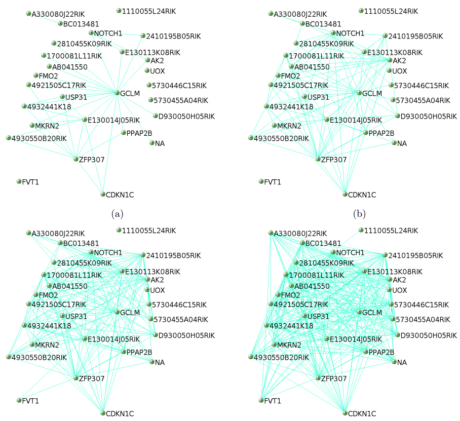
导出网络用于Cytoscape
- probes = colnames(dataExpr)
- dimnames(TOM) <- list(probes, probes)
- # Export the network into edge and node list files Cytoscape can read
- # threshold 默认为0.5, 可以根据自己的需要调整,也可以都导出后在
- # cytoscape中再调整
- cyt = exportNetworkToCytoscape(TOM,
- edgeFile = paste(exprMat, ".edges.txt", sep=""),
- nodeFile = paste(exprMat, ".nodes.txt", sep=""),
- weighted = TRUE, threshold = 0,
- nodeNames = probes, nodeAttr = moduleColors)
关联表型数据
- trait <- "WGCNA/TraitsClean.txt"
- # 读入表型数据,不是必须的
- if(trait != "") {
- traitData <- read.table(file=trait, sep='\t', header=T, row.names=1,
- check.names=FALSE, comment='',quote="")
- sampleName = rownames(dataExpr)
- traitData = traitData[match(sampleName, rownames(traitData)), ]
- }
- ### 模块与表型数据关联
- if (corType=="pearsoon") {
- modTraitCor = cor(MEs_col, traitData, use = "p")
- modTraitP = corPvalueStudent(modTraitCor, nSamples)
- } else {
- modTraitCorP = bicorAndPvalue(MEs_col, traitData, robustY=robustY)
- modTraitCor = modTraitCorP$bicor
- modTraitP = modTraitCorP$p
- }
- ## Warning in bicor(x, y, use = use, ...): bicor: zero MAD in variable 'y'.
- ## Pearson correlation was used for individual columns with zero (or missing)
- ## MAD.
- # signif表示保留几位小数
- textMatrix = paste(signif(modTraitCor, 2), "\n(", signif(modTraitP, 1), ")", sep = "")
- dim(textMatrix) = dim(modTraitCor)
- labeledHeatmap(Matrix = modTraitCor, xLabels = colnames(traitData),
- yLabels = colnames(MEs_col),
- cex.lab = 0.5,
- ySymbols = colnames(MEs_col), colorLabels = FALSE,
- colors = blueWhiteRed(50),
- textMatrix = textMatrix, setStdMargins = FALSE,
- cex.text = 0.5, zlim = c(-1,1),
- main = paste("Module-trait relationships"))
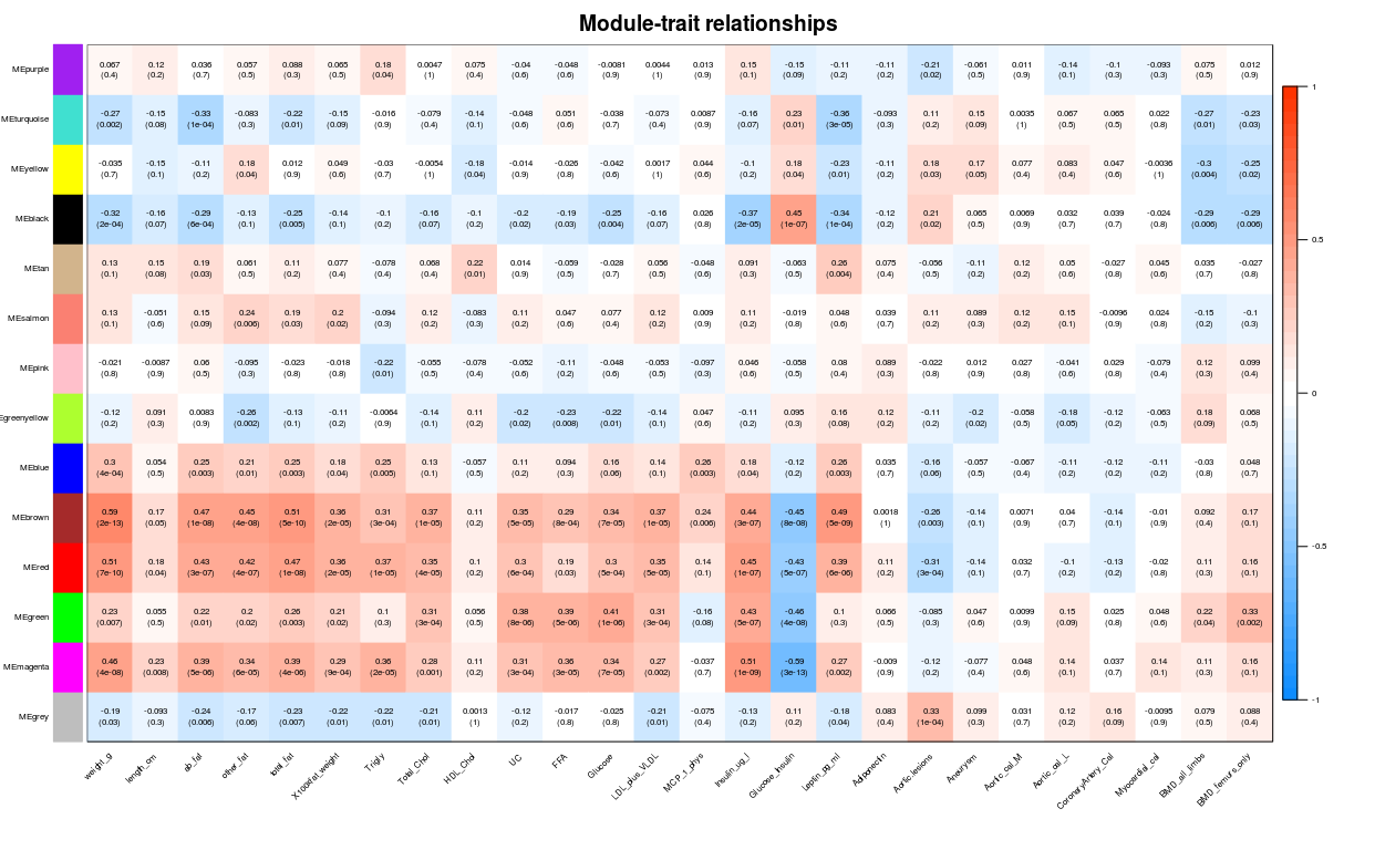
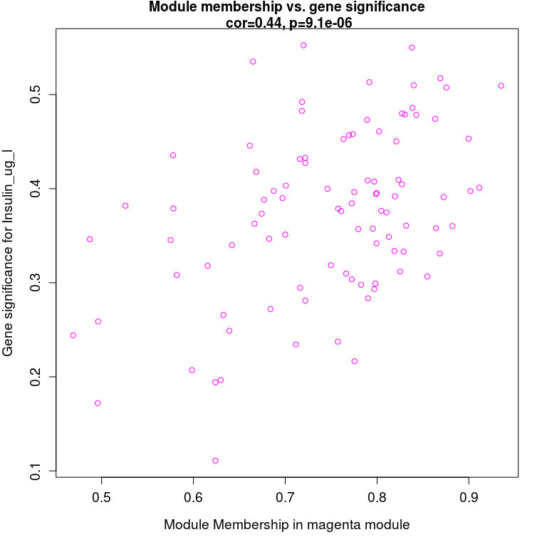
模块内基因与表型数据关联, 从上图可以看到MEmagenta与Insulin_ug_l相关,选取这两部分进行分析。
- ## 从上图可以看到MEmagenta与Insulin_ug_l相关
- ## 模块内基因与表型数据关联
- # 性状跟模块虽然求出了相关性,可以挑选最相关的那些模块来分析,
- # 但是模块本身仍然包含非常多的基因,还需进一步的寻找最重要的基因。
- # 所有的模块都可以跟基因算出相关系数,所有的连续型性状也可以跟基因的表达
- # 值算出相关系数。
- # 如果跟性状显著相关基因也跟某个模块显著相关,那么这些基因可能就非常重要
- # 。
- ### 计算模块与基因的相关性矩阵
- if (corType=="pearsoon") {
- geneModuleMembership = as.data.frame(cor(dataExpr, MEs_col, use = "p"))
- MMPvalue = as.data.frame(corPvalueStudent(
- as.matrix(geneModuleMembership), nSamples))
- } else {
- geneModuleMembershipA = bicorAndPvalue(dataExpr, MEs_col, robustY=robustY)
- geneModuleMembership = geneModuleMembershipA$bicor
- MMPvalue = geneModuleMembershipA$p
- }
- # 计算性状与基因的相关性矩阵
- ## 只有连续型性状才能进行计算,如果是离散变量,在构建样品表时就转为0-1矩阵。
- if (corType=="pearsoon") {
- geneTraitCor = as.data.frame(cor(dataExpr, traitData, use = "p"))
- geneTraitP = as.data.frame(corPvalueStudent(
- as.matrix(geneTraitCor), nSamples))
- } else {
- geneTraitCorA = bicorAndPvalue(dataExpr, traitData, robustY=robustY)
- geneTraitCor = as.data.frame(geneTraitCorA$bicor)
- geneTraitP = as.data.frame(geneTraitCorA$p)
- }
- ## Warning in bicor(x, y, use = use, ...): bicor: zero MAD in variable 'y'.
- ## Pearson correlation was used for individual columns with zero (or missing)
- ## MAD.
- # 最后把两个相关性矩阵联合起来,指定感兴趣模块进行分析
- module = "magenta"
- pheno = "Insulin_ug_l"
- modNames = substring(colnames(MEs_col), 3)
- # 获取关注的列
- module_column = match(module, modNames)
- pheno_column = match(pheno,colnames(traitData))
- # 获取模块内的基因
- moduleGenes = moduleColors == module
- sizeGrWindow(7, 7)
- par(mfrow = c(1,1))
- # 与性状高度相关的基因,也是与性状相关的模型的关键基因
- verboseScatterplot(abs(geneModuleMembership[moduleGenes, module_column]),
- abs(geneTraitCor[moduleGenes, pheno_column]),
- xlab = paste("Module Membership in", module, "module"),
- ylab = paste("Gene significance for", pheno),
- main = paste("Module membership vs. gene significance\n"),
- cex.main = 1.2, cex.lab = 1.2, cex.axis = 1.2, col = module)
分步法展示每一步都做了什么
- ### 计算邻接矩阵
- adjacency = adjacency(dataExpr, power = power)
- ### 把邻接矩阵转换为拓扑重叠矩阵,以降低噪音和假相关,获得距离矩阵。
- TOM = TOMsimilarity(adjacency)
- dissTOM = 1-TOM
- ### 层级聚类计算基因之间的距离树
- geneTree = hclust(as.dist(dissTOM), method = "average")
- ### 模块合并
- # We like large modules, so we set the minimum module size relatively high:
- minModuleSize = 30
- # Module identification using dynamic tree cut:
- dynamicMods = cutreeDynamic(dendro = geneTree, distM = dissTOM,
- deepSplit = 2, pamRespectsDendro = FALSE,
- minClusterSize = minModuleSize)
- # Convert numeric lables into colors
- dynamicColors = labels2colors(dynamicMods)
- ### 通过计算模块的代表性模式和模块之间的定量相似性评估,合并表达图谱相似
- 的模块
- MEList = moduleEigengenes(datExpr, colors = dynamicColors)
- MEs = MEList$eigengenes
- # Calculate dissimilarity of module eigengenes
- MEDiss = 1-cor(MEs)
- # Cluster module eigengenes
- METree = hclust(as.dist(MEDiss), method = "average")
- MEDissThres = 0.25
- # Call an automatic merging function
- merge = mergeCloseModules(datExpr, dynamicColors, cutHeight = MEDissThres, verbose = 3)
- # The merged module colors
- mergedColors = merge$colors;
- # Eigengenes of the new merged
- ## 分步法完结
1F
获取WGCNA
2F
获取WGCNA
3F
获取WGCNA
4F
获取WGCNA