

介绍完liger的数学原理,我们便可以来跑一跑liger的流程,并对liger的数学原理和参数选择有更深刻的理解。我们可以在GitHub上找到liger的码源以及相关的教程,本文也主要翻译自GitHub上的教程,并加入了一些自己的函数和理解。
载入包和数据
本文的教程希望整合控制组以及干扰素刺激组的PBMC单细胞RNA-seq数据,数据来源于Kang et al, 2017,liger的作者则提供了以RData格式存储的经过down sample的表达矩阵,我们可以从这里下载并直接使用。当然,如果你使用10x的数据的话,则也可以使用read10X函数将数据读入。
- ############################################
- ## Project: Liger-learning
- ## Script Purpose: run pipeline of liger integration and further analysis
- ## Data: 2020.10.24
- ## Author: Yiming Sun
- ############################################
- # general setting
- setwd('/data/User/sunym/project/liger_learning/')
- # library
- library(liger)
- library(Seurat)
- library(dplyr)
- library(tidyverse)
- library(viridis)
- library(parallel)
- #my function
- MySuggestLambda <- function(object,lambda,k,knn_k = 20,thresh = 1e-04,max.iters = 100,k2 = 500,ref_dataset = NULL,resolution = 1,parl_num){
- res <- matrix(ncol = 2,nrow = length(lambda))
- colnames(res) <- c('lambda','alignment')
- res[,'lambda'] <- lambda
- cl <- makeCluster(parl_num)
- clusterExport(cl,c('object','k','knn_k','thresh','max.iters','k2','ref_dataset','resolution'),envir = environment())
- clusterExport(cl,c('optimizeALS','quantileAlignSNF','calcAlignment'),envir = .GlobalEnv)
- alignment_score <- parLapply(cl = cl,lambda,function(x){
- object <- optimizeALS(object,k = k,lambda = x,thresh = thresh,max.iters = max.iters)
- object <- quantileAlignSNF(object,knn_k = knn_k,k2 = k2,ref_dataset = ref_dataset,resolution = resolution)
- return(calcAlignment(object))
- })
- stopCluster(cl)
- res[,'alignment'] <- (alignment_score %>% unlist())
- res <- as.data.frame(res)
- res[,1] <- as.numeric(as.character(res[,1]))
- res[,2] <- as.numeric(as.character(res[,2]))
- p <- ggplot(res,aes(x = lambda,y = alignment)) geom_point() geom_line()
- return(list(res,p))
- }
- # 1.Integrating Multiple Single-Cell RNA-seq Datasets
- #load data
- ctrl_dge <- readRDS("./data/PBMC_control.RDS")
- stim_dge <- readRDS("./data/PBMC_interferon-stimulated.RDS")
这里我写了一个函数MySuggestLambda用来优化λ的选择,其实liger包自带有suggestK和suggestLambda函数帮助我们优化K和λ的选择,但是suggestLambda函数似乎有什么bug,在一台服务器上跑完优化后会报一个莫名其妙的错误,而在另一台服务器上则完全正常,我还没有发现bug在哪里所以就自己写了个类似的函数帮助我优化λ的选择,如果你使用liger默认的函数也会报错的话不妨试试我的函数,虽然他内存运用效率特别低,建议配置好50G左右的swap区,因为当R跑多线程时,如果内存不够rsession会被直接挤掉,配置好swap能拯救一下它(血泪教训)。
标准化
在降维和聚类(整合)之前,我们通常都要对表达矩阵进行标准化、挑选variable gene最后再归一化。需要注意的是,liger使用的是非负矩阵分解的方法,因此我们在做归一化的时候注意不要做中心化,因为这会导致负数的出现。
- #initialize a liger object
- ifnb_liger <- createLiger(list(ctrl = ctrl_dge, stim = stim_dge))
- #explore liger object
- dim([email protected]$ctrl)
- head(colnames([email protected]$ctrl))
- head(rownames([email protected]$ctrl))
- dim([email protected]$stim)
- #normalize data
- ifnb_liger <- normalize(ifnb_liger)
- #select variable gene
- ifnb_liger <- selectGenes(ifnb_liger)
- #scale data but not center
- ifnb_liger <- scaleNotCenter(ifnb_liger)
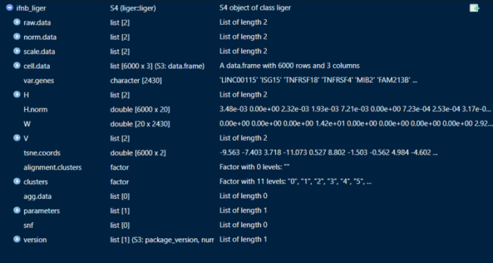
可以简单关注一下liger的数据结构,原始的表达矩阵存储在raw.data中,聚类的信息存储在clusters中,降维的信息存储在tsne.coords中。这里就不得不提一下seurat,seurat有一个meta.data的表格来存储各个细胞的各种信息,因此在我们做个性化的比较分析的时候特别有用。liger虽然也有cell.data,但我们似乎不太能够利用liger自带的函数指定cell.data中的变量来进行比较,我想到的解决方法是把liger导出为seurat,在seurat中做一些个性化的比较,而liger则单纯用来做整合、降维以及聚类。
非负矩阵分解
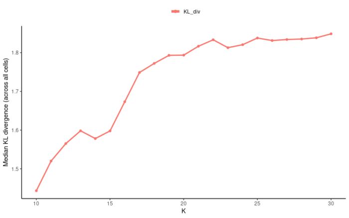
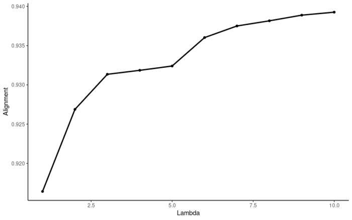
Liger利用非负矩阵分解的方法进行数据集之间的整合,我们需要提供的参数为K和λ。通常,K反映了数据集中真实cluster的个数,而λ则反映了数据集之间的异质性,如果你对你的数据完全没有把握,那么默认参数K=20,λ=5往往也能有不错的表现。当然我们也可以根据KL散度和Alignment score来优化K和λ的选择。
- #find the optimized k
- suggestK(ifnb_liger,k.test = seq(10,30,1),lambda = 5,plot.log2 = FALSE,num.cores = 10)
设置λ=5,调用10个进程,测试K从10到30时所计算得到的KL散度,最终选择20作为最优的K。
使用liger自带的函数优化λ的选择,取K=20,测试lambda的范围从1到10,调用10个进程,最终选择5作为最优的λ。
- #find the optimized lambda
- #use liger function
- suggestLambda(object = ifnb_liger,k = 20,lambda.test = seq(1,10,1),num.cores = 10)
使用我自己写的函数来优化λ的选择,
- #use my function
- suggest_lambda <- MySuggestLambda(ifnb_liger,lambda = seq(1,10,1),k = 20,parl_num = 10)
- suggest_lambda[[2]]
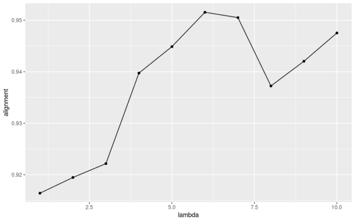
官方的函数应该是在Alignment score上做了平均而使得曲线更加平滑了,总之建议使用官方的函数,如果出现报错的话,可以试试我的函数。最后我们选择K=20,λ=5进行非负矩阵分解。
- #use lambda 5 k 20
- #integrate NMF
- ifnb_liger <- optimizeALS(ifnb_liger,k = 20,lambda = 5,max.iters = 30,thresh = 1e-06)
聚类
做完非负矩阵分解后就可以进行聚类了,liger聚类的方法也比较有趣,可以参考liger的数学原理。quantile_norm函数会构建SFN图(shared factor neighborhood graph)对细胞进行聚类,在聚类完成后将同一cluster中不同数据集来源的细胞在坐标轴(W V矩阵)上进行分位数归一化。
- #Quantile Normalization and Joint Clustering
- ifnb_liger <- quantile_norm(ifnb_liger,knn_k = 20,quantiles = 50,min_cells = 20,do.center = FALSE,
- max_sample = 1000,refine.knn = TRUE,eps = 0.9)
这里需要讲两个参数,knn_k是在构建SFN图中选择邻居细胞的个数,do.center是指是否做中心化,一般默认为FALSE,但当我们处理一些比较dense的数据时,如DNA甲基化数据,metagene的loading值通常会很高,此时可以做一下中心化来进行矫正。当然,我们也可以用一些图聚类算法来进一步优化我们的聚类,这一步可做可不做。
- # you can use louvain cluster to detect and assign cluster
- ifnb_liger <- louvainCluster(ifnb_liger, resolution = 0.25)
可视化与下游分析
- UMAP降维图
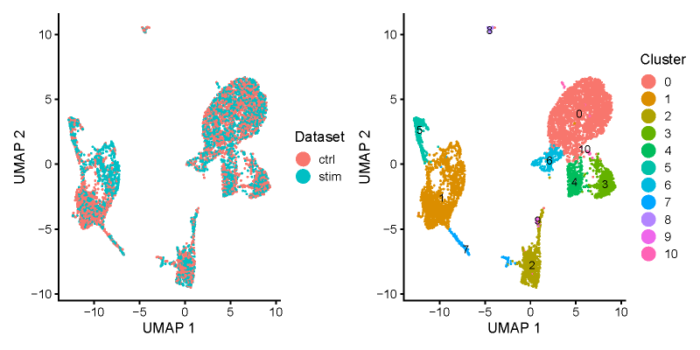
- #Visualization and Downstream Analysis
- ifnb_liger <- runUMAP(ifnb_liger, distance = 'cosine', n_neighbors = 30, min_dist = 0.3)
- all.plots <- plotByDatasetAndCluster(ifnb_liger, axis.labels = c('UMAP 1', 'UMAP 2'), return.plots = T)
- all.plots[[1]] all.plots[[2]]
- Gene loading plot
我们可以找到在各个cluster中高表达的metagene,以及这些metagene在不同的数据集中(W和V矩阵)对其贡献最高的基因。
- #find the maximun loading factor on each cluster and the maximun loading gene on the factor
- gene_loadings <- plotGeneLoadings(ifnb_liger, do.spec.plot = FALSE, return.plots = TRUE)
- gene_loadings[[4]]
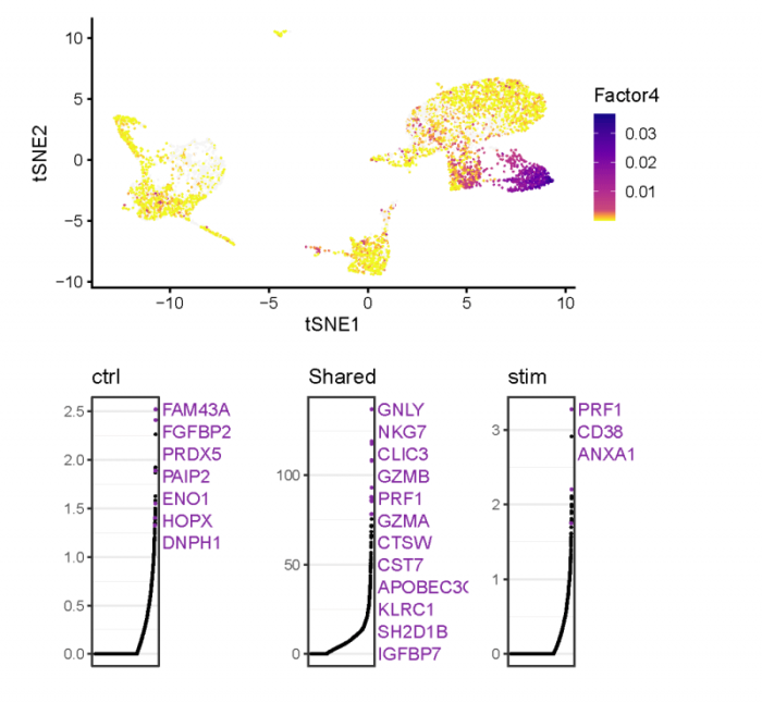
metagene_4在cluster_3中特异性高表达,那么metagene_4在W矩阵中对其贡献最大的基因(Shared),则很有可能是cluster_3的marker基因。类似的,metagene_4在V矩阵中对其贡献最大的基因,则反映了同一细胞类型数据集之间(或处理之间)的差异。我们也可以很容易得到图片背后的数据。
- #the metadata of the factor/gene loading plot
- #UMAP
- head(gene_loadings[[4]][[1]]$data)
- #gene loading value on the specific factor
- head(gene_loadings[[4]][[2]][[1]]$data[order(gene_loadings[[4]][[2]][[1]]$data$loadings,decreasing = TRUE),])
- head(gene_loadings[[4]][[2]][[2]]$data[order(gene_loadings[[4]][[2]][[2]]$data$loadings,decreasing = TRUE),])
- head(gene_loadings[[4]][[2]][[3]]$data[order(gene_loadings[[4]][[2]][[3]]$data$loadings,decreasing = TRUE),])
- # conclusion: gene_loadings object is a list of all the factor, specific the factor you want
- # conclusion: the factor object listed by gene_loadings has two lists, the first is the UMAP with the factor loading value, the second is the dataset-sepcific matrix W
- # the dataset specific matrix W is a list contains the all the dataset and shared gene loading value
- # what a mess!
总之就是list套list,很麻烦,可以对照着图和输出理解一下。
- > head(gene_loadings[[4]][[1]]$data)
- Factor4 tSNE1 tSNE2
- ctrlTCAGCGCTGGTCAT-1 0.0018384202 -9.5633178 -1.5025842
- ctrlTTATGGCTTCATTC-1 NA -7.4026990 -0.5618219
- ctrlACCCACTGCTTAGG-1 0.0007611497 3.7179575 4.9839707
- ctrlATGGGTACCCCGTT-1 0.0001820607 -11.0730367 -4.6024990
- ctrlTGACTGGACAGTCA-1 NA 0.5273923 -8.4171533
- ctrlGTGTAGTGGTTGTG-1 0.0013735353 8.8018236 5.2826267
- > #gene loading value on the specific factor
- > head(gene_loadings[[4]][[2]][[1]]$data[order(gene_loadings[[4]][[2]][[1]]$data$loadings,decreasing = TRUE),])
- loadings xpos top_k
- FAM43A 2.522310 1.0000000 TRUE
- FGFBP2 2.411532 0.9995883 TRUE
- SPON2 2.264957 0.9991766 FALSE
- ZNF638 1.925689 0.9987649 FALSE
- KARS 1.916834 0.9983532 FALSE
- PRDX5 1.889175 0.9979415 TRUE
- > head(gene_loadings[[4]][[2]][[2]]$data[order(gene_loadings[[4]][[2]][[2]]$data$loadings,decreasing = TRUE),])
- loadings xpos top_k
- GNLY 136.98236 1.0000000 TRUE
- NKG7 119.07990 0.9995883 TRUE
- CLIC3 117.71097 0.9991766 TRUE
- GZMB 108.58467 0.9987649 TRUE
- PRF1 108.14754 0.9983532 TRUE
- GZMA 93.22887 0.9979415 TRUE
- > head(gene_loadings[[4]][[2]][[3]]$data[order(gene_loadings[[4]][[2]][[3]]$data$loadings,decreasing = TRUE),])
- loadings xpos top_k
- PRF1 3.273654 1.0000000 TRUE
- SDF2L1 2.913147 0.9995883 FALSE
- CD38 2.204181 0.9991766 TRUE
- IFNG 2.111837 0.9987649 FALSE
- HSPA5 2.081298 0.9983532 FALSE
- CIAPIN1 2.002635 0.9979415 FALSE
- 差异表达分析
转录组分析怎么离得开差异表达分析嘛,我们可以用runWilcoxon比较不同的cluster之间的差异表达基因,也可以比较同一个cluster的不同数据集来源之间的差异表达基因。
- #differential gene express
- # for different cluster
- cluster.results <- runWilcoxon(ifnb_liger, compare.method = "clusters")
- head(cluster.results)
- datasets.results <- runWilcoxon(ifnb_liger, compare.method = "datasets")
- head(datasets.results)
只需要指定compare.method就可以进行不同的比较,不过这个函数其实也只能做这两种比较,如果我想做之前提到的更加个性化的比较,就只能导入到seurat中再进行比较。
- > cluster.results <- runWilcoxon(ifnb_liger, compare.method = "clusters")
- [1] "Performing Wilcoxon test on ALL datasets: ctrl, stim"
- > head(cluster.results)
- feature group avgExpr logFC statistic
- 1 RP11-206L10.2 0 -23.01898 -0.005557170 4259604
- 2 RP11-206L10.9 0 -23.01914 -0.005979592 4259602
- 3 LINC00115 0 -23.00609 -0.031260202 4252898
- 4 NOC2L 0 -21.83167 0.292228474 4340248
- 5 KLHL17 0 -23.00556 0.003658342 4262141
- 6 PLEKHN1 0 -23.01194 -0.039663835 4249915
- auc pval padj pct_in pct_out
- 1 0.4998057 0.570575909 0.69419204 100 100
- 2 0.4998055 0.570110484 0.69419204 100 100
- 3 0.4990189 0.138680541 0.24813295 100 100
- 4 0.5092682 0.004585054 0.01435755 100 100
- 5 0.5001034 0.819517383 0.88363326 100 100
- 6 0.4986689 0.044537037 0.10099905 100 100
- > datasets.results <- runWilcoxon(ifnb_liger, compare.method = "datasets")
- [1] "Performing Wilcoxon test on ALL datasets: ctrl, stim"
- > head(datasets.results)
- feature group avgExpr logFC statistic
- 1 RP11-206L10.2 0-ctrl -23.02585 -0.01408078 665437.5
- 2 RP11-206L10.9 0-ctrl -23.02585 -0.01376717 665437.5
- 3 LINC00115 0-ctrl -22.99983 0.01283157 666564.5
- 4 NOC2L 0-ctrl -21.87312 -0.08498766 662383.5
- 5 KLHL17 0-ctrl -22.98625 0.03960509 667718.0
- 6 PLEKHN1 0-ctrl -23.02585 -0.02853147 664846.0
- auc pval padj pct_in pct_out
- 1 0.4995560 0.30577296 0.6990712 100 100
- 2 0.4995560 0.30577296 0.6990712 100 100
- 3 0.5004020 0.59231247 0.8964793 100 100
- 4 0.4972633 0.61893894 0.9110340 100 100
- 5 0.5012680 0.09102028 0.4580475 100 100
- 6 0.4991119 0.14726281 0.5773302 100 100
对差异表达进行筛选。
- > # filter the data to find the meaningful DEG for your own experiment
- > cluster.results <- cluster.results[cluster.results$padj < 0.05,]
- > cluster.results <- cluster.results[cluster.results$logFC > 3,]
- > wilcoxon.cluster_3 <- cluster.results[cluster.results$group == 3, ]
- > wilcoxon.cluster_3 <- wilcoxon.cluster_3[order(wilcoxon.cluster_3$padj), ]
- > markers <- wilcoxon.cluster_3[1:20, ]
- > head(markers)
- feature group avgExpr logFC statistic auc
- 41861 GNLY 3 -5.282466 16.147323 2379942 0.9647642
- 46904 CLIC3 3 -12.962070 9.485599 1946458 0.7890417
- 47130 PRF1 3 -12.260573 9.830082 1970124 0.7986352
- 49239 GZMB 3 -7.840488 13.697178 2231966 0.9047789
- 52832 NKG7 3 -6.594620 14.433185 2324832 0.9424243
- 48310 KLRC1 3 -18.000059 4.916239 1606731 0.6513252
- pval padj pct_in pct_out
- 41861 0.000000e 00 0.000000e 00 100 100
- 46904 0.000000e 00 0.000000e 00 100 100
- 47130 0.000000e 00 0.000000e 00 100 100
- 49239 0.000000e 00 0.000000e 00 100 100
- 52832 0.000000e 00 0.000000e 00 100 100
- 48310 1.839405e-289 4.099114e-286 100 100
可以看一下PRF1在不同的cluster之间的表达情况。
- # feature plot on UMAP
- PRF1 <- plotGene(ifnb_liger, "PRF1", axis.labels = c('UMAP 1', 'UMAP 2'), return.plots = T)
- PRF1[[1]] PRF1[[2]]
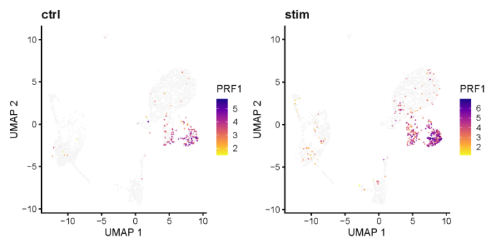
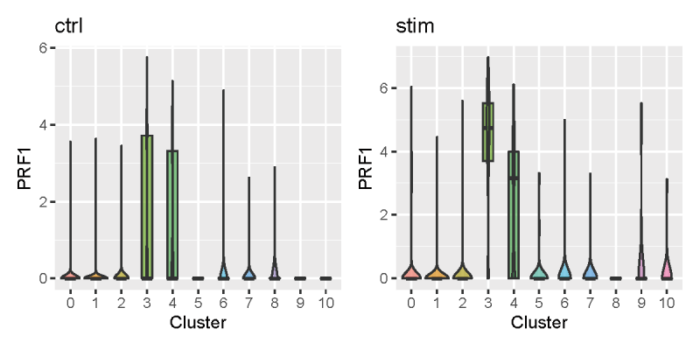
可以看到PRF1在两个数据集的cluster_3中均显著高表达。也可以用小提琴图来展示。
- # vlnplot
- PRF1 <- plotGeneViolin(ifnb_liger,gene = 'PRF1',return.plots = TRUE)
- PRF1[[1]] PRF1[[2]]
完整代码
- ############################################
- ## Project: Liger-learning
- ## Script Purpose: run pipeline of liger integration and further analysis
- ## Data: 2020.10.24
- ## Author: Yiming Sun
- ############################################
- # general setting
- setwd('/data/User/sunym/project/liger_learning/')
- # library
- library(liger)
- library(Seurat)
- library(dplyr)
- library(tidyverse)
- library(viridis)
- library(parallel)
- #my function
- MySuggestLambda <- function(object,lambda,k,knn_k = 20,thresh = 1e-04,max.iters = 100,k2 = 500,ref_dataset = NULL,resolution = 1,parl_num){
- res <- matrix(ncol = 2,nrow = length(lambda))
- colnames(res) <- c('lambda','alignment')
- res[,'lambda'] <- lambda
- cl <- makeCluster(parl_num)
- clusterExport(cl,c('object','k','knn_k','thresh','max.iters','k2','ref_dataset','resolution'),envir = environment())
- clusterExport(cl,c('optimizeALS','quantileAlignSNF','calcAlignment'),envir = .GlobalEnv)
- alignment_score <- parLapply(cl = cl,lambda,function(x){
- object <- optimizeALS(object,k = k,lambda = x,thresh = thresh,max.iters = max.iters)
- object <- quantileAlignSNF(object,knn_k = knn_k,k2 = k2,ref_dataset = ref_dataset,resolution = resolution)
- return(calcAlignment(object))
- })
- stopCluster(cl)
- res[,'alignment'] <- (alignment_score %>% unlist())
- res <- as.data.frame(res)
- res[,1] <- as.numeric(as.character(res[,1]))
- res[,2] <- as.numeric(as.character(res[,2]))
- p <- ggplot(res,aes(x = lambda,y = alignment)) geom_point() geom_line()
- return(list(res,p))
- }
- # 1.Integrating Multiple Single-Cell RNA-seq Datasets
- #load data
- ctrl_dge <- readRDS("./data/PBMC_control.RDS")
- stim_dge <- readRDS("./data/PBMC_interferon-stimulated.RDS")
- #initialize a liger object
- ifnb_liger <- createLiger(list(ctrl = ctrl_dge, stim = stim_dge))
- #explore liger object
- dim([email protected]$ctrl)
- head(colnames([email protected]$ctrl))
- head(rownames([email protected]$ctrl))
- dim([email protected]$stim)
- #normalize data
- ifnb_liger <- normalize(ifnb_liger)
- #select variable gene
- ifnb_liger <- selectGenes(ifnb_liger)
- #scale data but not center
- ifnb_liger <- scaleNotCenter(ifnb_liger)
- #find the optimized k
- suggestK(ifnb_liger,k.test = seq(10,30,1),lambda = 5,plot.log2 = FALSE,num.cores = 10)
- #find the optimized lambda
- #use liger function
- suggestLambda(object = ifnb_liger,k = 20,lambda.test = seq(1,10,1),num.cores = 10)
- #use my function
- suggest_lambda <- MySuggestLambda(ifnb_liger,lambda = seq(1,10,1),k = 20,parl_num = 10)
- suggest_lambda[[2]]
- #use lambda 5 k 20
- #integrate NMF
- ifnb_liger <- optimizeALS(ifnb_liger,k = 20,lambda = 5,max.iters = 30,thresh = 1e-06)
- #Quantile Normalization and Joint Clustering
- ifnb_liger <- quantile_norm(ifnb_liger,knn_k = 20,quantiles = 50,min_cells = 20,do.center = FALSE,
- max_sample = 1000,refine.knn = TRUE,eps = 0.9)
- # you can use louvain cluster to detect and assign cluster
- ifnb_liger <- louvainCluster(ifnb_liger, resolution = 0.25)
- head([email protected])
- #Visualization and Downstream Analysis
- ifnb_liger <- runUMAP(ifnb_liger, distance = 'cosine', n_neighbors = 30, min_dist = 0.3)
- all.plots <- plotByDatasetAndCluster(ifnb_liger, axis.labels = c('UMAP 1', 'UMAP 2'), return.plots = T)
- #the place of each cell and the cluster it belongs
- head(all.plots[[1]]$data)
- pdf(file = './res/fig_201024/plot_by_dataset_and_cluster.pdf',width = 8,height = 4)
- all.plots[[1]] all.plots[[2]]
- dev.off()
- #find the maximun loading factor on each cluster and the maximun loading gene on the factor
- gene_loadings <- plotGeneLoadings(ifnb_liger, do.spec.plot = FALSE, return.plots = TRUE)
- pdf(file = './res/fig_201024/gene_loading_plot.pdf',width = 6.5,height = 6)
- gene_loadings[[4]]
- dev.off()
- #the metadata of the factor/gene loading plot
- #UMAP
- head(gene_loadings[[4]][[1]]$data)
- #gene loading value on the specific factor
- head(gene_loadings[[4]][[2]][[1]]$data[order(gene_loadings[[4]][[2]][[1]]$data$loadings,decreasing = TRUE),])
- head(gene_loadings[[4]][[2]][[2]]$data[order(gene_loadings[[4]][[2]][[2]]$data$loadings,decreasing = TRUE),])
- head(gene_loadings[[4]][[2]][[3]]$data[order(gene_loadings[[4]][[2]][[3]]$data$loadings,decreasing = TRUE),])
- # conclusion: gene_loadings object is a list of all the factor, specific the factor you want
- # conclusion: the factor object listed by gene_loadings has two lists, the first is the UMAP with the factor loading value, the second is the dataset-sepcific matrix W
- # the dataset specific matrix W is a list contains the all the dataset and shared gene loading value
- # what a mess!
- #differential gene express
- # for different cluster
- cluster.results <- runWilcoxon(ifnb_liger, compare.method = "clusters")
- head(cluster.results)
- datasets.results <- runWilcoxon(ifnb_liger, compare.method = "datasets")
- head(datasets.results)
- # filter the data to find the meaningful DEG for your own experiment
- cluster.results <- cluster.results[cluster.results$padj < 0.05,]
- cluster.results <- cluster.results[cluster.results$logFC > 3,]
- wilcoxon.cluster_3 <- cluster.results[cluster.results$group == 3, ]
- wilcoxon.cluster_3 <- wilcoxon.cluster_3[order(wilcoxon.cluster_3$padj), ]
- markers <- wilcoxon.cluster_3[1:20, ]
- head(markers)
- # feature plot on UMAP
- PRF1 <- plotGene(ifnb_liger, "PRF1", axis.labels = c('UMAP 1', 'UMAP 2'), return.plots = T)
- pdf(file = './res/fig_201024/feature_plot_PRF1.pdf',width = 8,height = 4)
- PRF1[[1]] PRF1[[2]]
- dev.off()
- # vlnplot
- PRF1 <- plotGeneViolin(ifnb_liger,gene = 'PRF1',return.plots = TRUE)
- pdf(file = './res/fig_201024/vlnplot_PRF1.pdf',width = 6,height = 3)
- PRF1[[1]] PRF1[[2]]
- dev.off()
- # compare cluster marker express winthin and across dataset
- IFIT3 <- plotGene(ifnb_liger, "IFIT3", axis.labels = c('UMAP 1', 'UMAP 2'), return.plots = TRUE)
- IFITM3 <- plotGene(ifnb_liger, "IFITM3", axis.labels = c('UMAP 1', 'UMAP 2'), return.plots = TRUE)
- pdf(file = './res/fig_201024/cluster_marker_within_between_dataset.pdf',width = 8,height = 8)
- plot_grid(IFIT3[[1]],IFIT3[[2]],IFITM3[[1]],IFITM3[[2]], ncol=2)
- dev.off()