

1 Rle(Run Length Encoding,行程编码)
1.1 Rle类和Rle对象
序列或基因最终要定位到染色体上。序列往往数量非常巨大,但染色体数量很少,如果每条序列的染色体定位都显式标注,将会产生大量的重复信息,更糟糕的是它们要占用大量的内存。BioC的IRanges包为这些数据提供了一种简便可行的信息压缩方式,即Rle。如果染色体1-3分别有3000,5000和2000个基因,基因的染色体注释可以用字符向量表示,也可以用Rle对象表示:
- library(IRanges) #可以不执行,载入Biostrings包将自动载入依赖包IRanges
- library(Biostrings)
- chr.str <- c(rep("ChrI", 3000), rep("ChrII", 5000), rep("ChrIII", 2000))
- chr.rle <- Rle(chr.str)
两种方式的效果是完全一样的,但是Rle对象占用空间还不到字符向量的2%:
- # Rle对象向量化后和原向量是完全相同的
- identical(as.vector(chr.rle), chr.str)
- ## [1] TRUE
- # 对象大小(内存占用)比:
- as.vector(object.size(chr.rle)/object.size(chr.str))
- ## [1] 0.01795
使用Rle并不总是可以“压缩”数据。如果信息没有重复或重复量很少,Rle会占用更多的内存:
- strx <- sample(DNA_BASES, 10000, replace = TRUE)
- strx.rle <- Rle(strx)
- as.vector(object.size(strx.rle)/object.size(strx))
- ## [1] 1.518
Rle对象用两个属性来表示原向量,一个是值(values),可以是向量或因子;另一个是长度(lengths),为整型数据,表示对应位置的value的重复次数。
- chr.rle
- ## character-Rle of length 10000 with 3 runs
- ## Lengths: 3000 5000 2000
- ## Values : "ChrI" "ChrII" "ChrIII"
- getClass(class(chr.rle))
- ## Class "Rle" [package "IRanges"]
- ##
- ## Slots:
- ##
- ## Name: values lengths elementMetadata metadata
- ## Class: vectorORfactor integer DataTableORNULL list
- ##
- ## Extends:
- ## Class "Vector", directly
- ## Class "Annotated", by class "Vector", distance 2
1.2 Rle对象的处理方法
1.2.1 Rle对象构建/获取
Rle对象可以用构造函数Rle来产生,它有两种用法:
- Rle(values)
- Rle(values, lengths)
values和lengths均为(原子)向量。第一种用法前面已经出现过了,我们看看第二种用法:
- chr.rle <- Rle(values = c("Chr1", "Chr2", "Chr3", "Chr1", "Chr3"), lengths = c(3,
- 2, 5, 4, 5))
- chr.rle
- ## character-Rle of length 19 with 5 runs
- ## Lengths: 3 2 5 4 5
- ## Values : "Chr1" "Chr2" "Chr3" "Chr1" "Chr3"
原子向量也可以通过类型转换函数as由原子向量产生,它等价于上面的第一种方式:
- as(chr.str, "Rle")
- ## character-Rle of length 10000 with 3 runs
- ## Lengths: 3000 5000 2000
- ## Values : "ChrI" "ChrII" "ChrIII"
1.2.2 获取属性
Rle是S4类,Rle对象的属性如值、长度等可以使用属性读取函数获取:
- runLength(chr.rle)
- ## [1] 3 2 5 4 5
- runValue(chr.rle)
- ## [1] "Chr1" "Chr2" "Chr3" "Chr1" "Chr3"
- nrun(chr.rle)
- ## [1] 5
- start(chr.rle)
- ## [1] 1 4 6 11 15
- end(chr.rle)
- ## [1] 3 5 10 14 19
- width(chr.rle)
- ## [1] 3 2 5 4 5
1.2.3 属性替换
Rle对象的长度和值还可以使用属性替换函数进行修改:
- runLength(chr.rle) <- rep(3, nrun(chr.rle))
- chr.rle
- ## character-Rle of length 15 with 5 runs
- ## Lengths: 3 3 3 3 3
- ## Values : "Chr1" "Chr2" "Chr3" "Chr1" "Chr3"
- runValue(chr.rle)[3:4] <- c("III", "IV")
- chr.rle
- ## character-Rle of length 15 with 5 runs
- ## Lengths: 3 3 3 3 3
- ## Values : "Chr1" "Chr2" "III" "IV" "Chr3"
- # 替换向量和被替换向量的长度必需相同,否则出错。下面两个语句都不正确:
- runValue(chr.rle) <- c("ChrI", "ChrV")
- ## Error: 'length(lengths)' != 'length(values)'
- runLength(chr.rle) <- 3
- ## Error: 'length(lengths)' != 'length(values)'
1.2.4 类型转换
除使用as.vector函数外,Rle对象还可以使用很多函数进行类型转换,如:
- as.factor(chr.rle)
- ## [1] Chr1 Chr1 Chr1 Chr2 Chr2 Chr2 III III III IV IV IV Chr3 Chr3
- ## [15] Chr3
- ## Levels: Chr1 Chr2 Chr3 III IV
- as.character(chr.rle)
- ## [1] "Chr1" "Chr1" "Chr1" "Chr2" "Chr2" "Chr2" "III" "III" "III" "IV"
- ## [11] "IV" "IV" "Chr3" "Chr3" "Chr3"
1.2.5 Rle的S4类集团泛函数运算
Rle是BioC定义的基础数据类型。既然“基础”,那么它应当能进行R语言中数据的一般性运算,比如加减乘除、求模、求余等数学运算。事实也是如此,Rle支持R语言S4类集团泛函数(group generic functions,“集团通用函数”?)运算,包括算术、复数、比较、逻辑、数学函数和R语言的汇总("max", "min", "range", "prod", "sum", "any", "all"等)运算(没有去验证是否所有运算都已实现)。下面仅简单具几个例子,具体情况请参考Rle-class的相关说明:
- set.seed(0)
- rle1 <- Rle(sample(4, 6, replace = TRUE))
- rle2 <- Rle(sample(5, 12, replace = TRUE))
- rle3 <- Rle(sample(4, 8, replace = TRUE))
- rle1 + rle2
- ## integer-Rle of length 12 with 11 runs
- ## Lengths: 1 1 1 1 1 1 1 1 1 2 1
- ## Values : 9 7 6 7 5 3 5 6 4 7 5
- rle1 + rle3
- ## integer-Rle of length 8 with 8 runs
- ## Lengths: 1 1 1 1 1 1 1 1
- ## Values : 8 4 6 7 5 4 5 4
- rle1 * rle2
- ## integer-Rle of length 12 with 11 runs
- ## Lengths: 1 1 1 1 1 1 1 1 1 2 1
- ## Values : 20 10 8 12 4 2 4 8 4 12 4
- sqrt(rle1)
- ## numeric-Rle of length 6 with 5 runs
- ## Lengths: 1 2 ... 1
- ## Values : 2 1.4142135623731 ... 1
- range(rle1)
- ## [1] 1 4
- cumsum(rle1)
- ## integer-Rle of length 6 with 6 runs
- ## Lengths: 1 1 1 1 1 1
- ## Values : 4 6 8 11 15 16
- (rle1 <- Rle(sample(DNA_BASES, 10, replace = TRUE)))
- ## character-Rle of length 10 with 9 runs
- ## Lengths: 1 1 1 1 2 1 1 1 1
- ## Values : "C" "A" "C" "T" "C" "G" "C" "A" "T"
- (rle2 <- Rle(sample(DNA_BASES, 8, replace = TRUE)))
- ## character-Rle of length 8 with 8 runs
- ## Lengths: 1 1 1 1 1 1 1 1
- ## Values : "G" "T" "A" "G" "C" "T" "G" "T"
- paste(rle1, rle2, sep = "")
- ## character-Rle of length 10 with 10 runs
- ## Lengths: 1 1 1 1 1 1 1 1 1 1
- ## Values : "CG" "AT" "CA" "TG" "CC" "CT" "GG" "CT" "AG" "TT"
2 Ranges(序列区间/范围)
2.1 BioC中的Ranges
Ranges是一类特殊但又常用的数据类型,它们可以表示小段序列在大段序列中的位置、名称和组织结构等信息。BioC中与Ranges定义有关的软件包主要有IRanges, GenomicRanges和GenomicFeatures。
IRanges包定义了Ranges的一般数据结构和处理方法,但不直接面向序列处理;GenomicRanges包定义的GRanges和GRangesList类除了储存Ranges信息外还包含了序列的名称和DNA链等信息;而GenomicFeatures(包)则处理以数据库形式提供的GRanges信息,如基因、外显子、内含子、启动子、UTR等。
先看看BioC中Ranges最基本的类定义:
- getClass("Ranges")
- ## Virtual Class "Ranges" [package "IRanges"]
- ##
- ## Slots:
- ##
- ## Name: elementType elementMetadata metadata
- ## Class: character DataTableORNULL list
- ##
- ## Extends:
- ## Class "IntegerList", directly
- ## Class "RangesORmissing", directly
- ## Class "AtomicList", by class "IntegerList", distance 2
- ## Class "List", by class "IntegerList", distance 3
- ## Class "Vector", by class "IntegerList", distance 4
- ## Class "Annotated", by class "IntegerList", distance 5
- ##
- ## Known Subclasses:
- ## Class "IRanges", directly
- ## Class "Partitioning", directly
- ## Class "GappedRanges", directly
- ## Class "IntervalTree", directly
- ## Class "NormalIRanges", by class "IRanges", distance 2
- ## Class "PartitioningByEnd", by class "Partitioning", distance 2
- ## Class "PartitioningByWidth", by class "Partitioning", distance 2
Ranges是虚拟类,实际应用中最常用的IRanges子类,它继承了Ranges的数据结构,另外多设置了3个slots(存储槽),分别用于存贮Ranges的起点、宽度和名称信息。由于Ranges由整数确定,所以称为IRanges(Integer Ranges,整数区间),但也有人理解成间隔区间(Interval Ranges):
- getSlots("Ranges")
- ## elementType elementMetadata metadata
- ## "character" "DataTableORNULL" "list"
- getSlots("IRanges")
- ## start width NAMES elementType
- ## "integer" "integer" "characterORNULL" "character"
- ## elementMetadata metadata
- ## "DataTableORNULL" "list"
GRanges是Ranges概念在序列处理上的具体应用,但它和IRanges没有继承关系:
- library(GenomicRanges)
- getSlots("GRanges")
- ## seqnames ranges strand elementMetadata
- ## "Rle" "IRanges" "Rle" "DataFrame"
- ## seqinfo metadata
- ## "Seqinfo" "list"
Ranges对于序列处理非常重要,除GenomicRanges外,Biostrings一些类的定义也应用了Ranges:
- getSlots("XStringViews")
- ## subject ranges elementType elementMetadata
- ## "XString" "IRanges" "character" "DataTableORNULL"
- ## metadata
- ## "list"
2.2 对象构建和属性获取
IRanges对象可以使用对象构造函数IRanges产生,需提供起点(start)、终点(end)和宽度(width)三个参数中的任意两个:
- ir1 <- IRanges(start = 1:10, width = 10:1)
- ir2 <- IRanges(start = 1:10, end = 11)
- ir3 <- IRanges(end = 11, width = 10:1)
- ir1
- ## IRanges of length 10
- ## start end width
- ## [1] 1 10 10
- ## [2] 2 10 9
- ## [3] 3 10 8
- ## [4] 4 10 7
- ## [5] 5 10 6
- ## [6] 6 10 5
- ## [7] 7 10 4
- ## [8] 8 10 3
- ## [9] 9 10 2
- ## [10] 10 10 1
GRanges对象也可以使用构造函数生成,其方式与数据框对象生成有些类似:
- genes <- GRanges(seqnames = c("Chr1", "Chr3", "Chr3"), ranges = IRanges(start = c(1300,
- 1050, 2000), end = c(2500, 1870, 3200)), strand = c("+", "+", "-"), seqlengths = c(Chr1 = 1e+05,
- Chr3 = 2e+05))
- genes
- ## GRanges with 3 ranges and 0 metadata columns:
- ## seqnames ranges strand
- ##
- ## [1] Chr1 [1300, 2500] +
- ## [2] Chr3 [1050, 1870] +
- ## [3] Chr3 [2000, 3200] -
- ## ---
- ## seqlengths:
- ## Chr1 Chr3
- ## 100000 200000
IRanges和GRanges都是S4类,其属性获取有相应的函数:
- start(ir1)
- ## [1] 1 2 3 4 5 6 7 8 9 10
- end(ir1)
- ## [1] 10 10 10 10 10 10 10 10 10 10
- width(ir1)
- ## [1] 10 9 8 7 6 5 4 3 2 1
- ranges(genes)
- ## IRanges of length 3
- ## start end width
- ## [1] 1300 2500 1201
- ## [2] 1050 1870 821
- ## [3] 2000 3200 1201
- start(ranges(genes))
- ## [1] 1300 1050 2000
Views对象也包含有IRanges属性:
- # 按长度设置产生随机序列的函数
- rndSeq <- function(dict, n) {
- paste(sample(dict, n, replace = T), collapse = "")
- }
- set.seed(0)
- dna <- DNAString(rndSeq(DNA_BASES, 1000))
- vws <- as(maskMotif(dna, "TGA"), "Views")
- (ir <- ranges(vws))
- ## IRanges of length 18
- ## start end width
- ## [1] 1 104 104
- ## [2] 108 264 157
- ## [3] 268 268 1
- ## [4] 272 300 29
- ## [5] 304 393 90
- ## ... ... ... ...
- ## [14] 586 752 167
- ## [15] 756 851 96
- ## [16] 855 912 58
- ## [17] 916 989 74
- ## [18] 993 1000 8
模式匹配的match类函数返回IRanges对象,而vmatch类函数返回GRanges类对象:
2.3 IRanges对象的运算和处理方法
2.3.1 Ranges内变换(Intra-range transformations)
这种类型的处理函数包括shift,flank,narrow,reflect,resize,restrict和promoters等,它们对每个Ranges进行独立处理。为了方便理解,我们使用IRanges包的Vignette提供的一个很有用的IRanges作图函数(稍做修改):
- plotRanges <- function(x, xlim = x, main = deparse(substitute(x)), col = "black",
- add = FALSE, ybottom = NULL, ...) {
- require(scales)
- col <- alpha(col, 0.5)
- height <- 1
- sep <- 0.5
- if (is(xlim, "Ranges")) {
- xlim <- c(min(start(xlim)), max(end(xlim)) * 1.2)
- }
- if (!add) {
- bins <- disjointBins(IRanges(start(x), end(x) + 1))
- ybottom <- bins * (sep + height) - height
- par(mar = c(3, 0.5, 2.5, 0.5), mgp = c(1.5, 0.5, 0))
- plot.new()
- plot.window(xlim, c(0, max(bins) * (height + sep)))
- }
- rect(start(x) - 0.5, ybottom, end(x) + 0.5, ybottom + height, col = col,
- ...)
- text((start(x) + end(x))/2, ybottom + height/2, 1:length(x), col = "white",
- xpd = TRUE)
- title(main)
- axis(1)
- invisible(ybottom)
- }
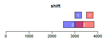
shift函数对Ranges进行平移(下面图形中蓝色为原始Ranges,红色为变换后的Ranges,黑色/灰色则为参考Ranges,其他颜色为重叠区域):
- ir <- IRanges(c(3000, 2500), width = c(300, 850))
- ir.trans <- shift(ir, 500)
- xlim <- c(0, max(end(ir, ir.trans)) * 1.3)
- ybottom <- plotRanges(ir, xlim = xlim, main = "shift", col = "blue")
- plotRanges(ir.trans, add = TRUE, ybottom = ybottom, main = "", col = "red")
flank函数获取Ranges的相邻区域,width参数为整数表示左侧,负数表示右侧:
- ir.trans <- flank(ir, width = 200)
- xlim <- c(0, max(end(ir, ir.trans)) * 1.3)
- ybottom <- plotRanges(ir, xlim = xlim, main = "flank", col = "blue")
- plotRanges(ir.trans, add = TRUE, ybottom = ybottom, main = "", col = "red")

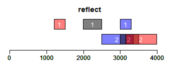
reflect函数获取Ranges的镜面对称区域,bounds为用于设置镜面位置的Ranges对象:
- bounds <- IRanges(c(2000, 3000), width = 500)
- ir.trans <- reflect(ir, bounds = bounds)
- xlim <- c(0, max(end(ir, ir.trans, bounds)) * 1.3)
- ybottom <- plotRanges(ir, xlim = xlim, main = "reflect", col = "blue")
- plotRanges(bounds, add = TRUE, ybottom = ybottom, main = "")
- plotRanges(ir.trans, add = TRUE, ybottom = ybottom, main = "", col = "red")
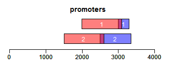
promoters函数获取promoter区域,upstream和downstream分别设置上游和下游截取的序列长度:
- ir.trans <- promoters(ir, upstream = 1000, downstream = 100)
- xlim <- c(0, max(end(ir, ir.trans)) * 1.3)
- ybottom <- plotRanges(ir, xlim = xlim, main = "promoters", col = "blue")
- plotRanges(ir.trans, add = TRUE, ybottom = ybottom, main = "", col = "red")
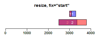
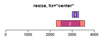
resize函数改变Ranges的大小,width设置宽度,fix设置固定位置(start/end/center):
- ir.trans <- resize(ir, width = c(100, 1300), fix = "start")
- xlim <- c(0, max(end(ir, ir.trans)) * 1.3)
- ybottom <- plotRanges(ir, xlim = xlim, main = "resize, fix=\"start\"", col = "blue")
- plotRanges(ir.trans, add = TRUE, ybottom = ybottom, main = "", col = "red")
- ir.trans <- resize(ir, width = c(100, 1300), fix = "center")
- xlim <- c(0, max(end(ir, ir.trans)) * 1.3)
- ybottom <- plotRanges(ir, xlim = xlim, main = "resize, fix=\"center\"", col = "blue")
- plotRanges(ir.trans, add = TRUE, ybottom = ybottom, main = "", col = "red")
其他函数的使用请自行尝试使用。
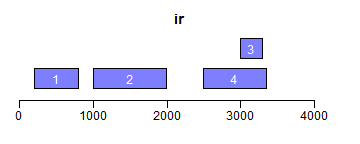
2.3.2 Ranges间转换(Inter-range transformations)
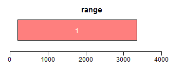
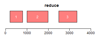
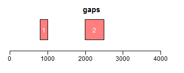
range函数用于获取Ranges所包括的整个区域(包括间隔区);reduce将重叠区域合并;gaps用于获取间隔区域:
- ir <- IRanges(c(200, 1000, 3000, 2500), width = c(600, 1000, 300, 850))
- ir.trans <- range(ir)
- xlim <- c(0, max(end(ir, ir.trans)) * 1.3)
- ybottom <- plotRanges(ir, xlim = xlim, col = "blue")
- plotRanges(ir.trans, xlim = xlim, col = "red", main = "range")
- ir.trans <- reduce(ir)
- plotRanges(ir.trans, xlim = xlim, col = "red", main = "reduce")
- ir.trans <- gaps(ir)
- plotRanges(ir.trans, xlim = xlim, col = "red", main = "gaps")
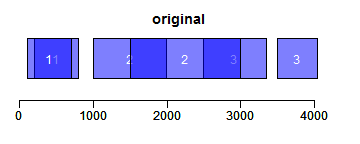
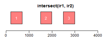
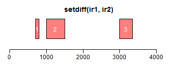
2.3.3 Ranges对象间的集合运算
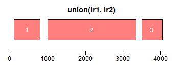
intersect求交集区域;setdiff求差异区域;union求并集:
- ir1 <- IRanges(c(200, 1000, 3000, 2500), width = c(600, 1000, 300, 850))
- ir2 <- IRanges(c(100, 1500, 2000, 3500), width = c(600, 800, 1000, 550))
- xlim <- c(0, max(end(ir1, ir2)) * 1.3)
- ybottom <- plotRanges(reduce(ir1), xlim = xlim, col = "blue", main = "original")
- plotRanges(reduce(ir2), xlim = xlim, col = "blue", main = "", add = TRUE, ybottom = ybottom)
- plotRanges(intersect(ir1, ir2), xlim = xlim, col = "red")
- plotRanges(setdiff(ir1, ir2), xlim = xlim, col = "red")
- plotRanges(union(ir1, ir2), xlim = xlim, col = "red")
此外还有punion,pintersect,psetdiff和pgap函数,进行element-wise的运算。
原文来自:http://blog.csdn.net/u014801157/article/details/24372479