用limma对芯片数据做差异分析

2013/09/15来源：生信菜鸟团1 35,187

用基因芯片的手段来探针基因表达量的技术虽然已经在逐步被RNA-seq技术取代，但毕竟经历了十多年的发展了，在GEO或arrayexpress数据库里面存储的全球研究者数据都已经超过了50PB了！实在是很可观，里面还是有非常多等待挖掘的地方！现在我们要讲的就是基因表达芯片数据的一种分析方式，差异分析，主角就是limma这个package，虽然一直都有各种差异分析统计方法提出来，但是limma包绝对是其中的佼佼者，我们也不多说废话了，直接上教程！

使用这个包需要三个数据：

表达矩阵
分组矩阵
差异比较矩阵

而且总共也只有三个步骤：

lmFit
eBayes
topTable

首先是表达矩阵，这个非常简单了，你可以自己从芯片原始的cel文件开始用affy包读取，然后用rma或者mas5函数做归一化处理，最后得到表达矩阵。也可以直接下载表达矩阵然后用read.table等函数读取到R里面。或者直接下载一个含有表达矩阵的数据对象！

suppressPackageStartupMessages(library(CLL))
data(sCLLex)
exprSet=exprs(sCLLex)   ##sCLLex是依赖于CLL这个package的一个对象
samples=sampleNames(sCLLex)
pdata=pData(sCLLex)
group_list=as.character(pdata[,2])
dim(exprSet)

## [1] 12625    22

exprSet[1:5,1:5]

##           CLL11.CEL CLL12.CEL CLL13.CEL CLL14.CEL CLL15.CEL
## 1000_at    5.743132  6.219412  5.523328  5.340477  5.229904
## 1001_at    2.285143  2.291229  2.287986  2.295313  2.662170
## 1002_f_at  3.309294  3.318466  3.354423  3.327130  3.365113
## 1003_s_at  1.085264  1.117288  1.084010  1.103217  1.074243
## 1004_at    7.544884  7.671801  7.474025  7.152482  6.902932

group_list  ##这个也是存储在sCLLex对象里面的信息，描述了样本的状态，需要根据它来进行样本分类

##  [1] "progres." "stable"   "progres." "progres." "progres." "progres."
##  [7] "stable"   "stable"   "progres." "stable"   "progres." "stable"  
## [13] "progres." "stable"   "stable"   "progres." "progres." "progres."
## [19] "progres." "progres." "progres." "stable"

可以看到我们得到了表达矩阵exprSet，它列是各个样本，行是每个探针ID，一个纯粹的表达矩阵，必须是数字型的！我们可以简单做该表达矩阵做一个QC检测。

par(cex = 0.7)
n.sample=ncol(exprSet)
if(n.sample>40) par(cex = 0.5)
cols <- rainbow(n.sample*1.2)
boxplot(exprSet, col = cols,main="expression value",las=2)

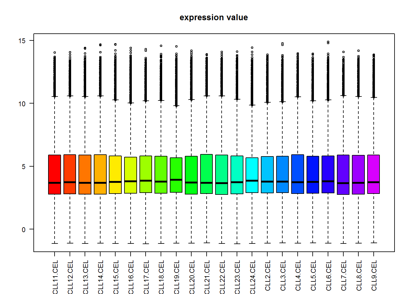
通过这些boxplot可以看到各个芯片直接数据还算整齐，可以进行差异比较

然后我们制作分组矩阵

suppressMessages(library(limma))

## Warning: package 'limma' was built under R version 3.1.1

design <- model.matrix(~0+factor(group_list))
colnames(design)=levels(factor(group_list))
rownames(design)=colnames(exprSet)
design

##           progres. stable
## CLL11.CEL        1      0
## CLL12.CEL        0      1
## CLL13.CEL        1      0
## CLL14.CEL        1      0
## CLL15.CEL        1      0
## CLL16.CEL        1      0
## CLL17.CEL        0      1
## CLL18.CEL        0      1
## CLL19.CEL        1      0
## CLL20.CEL        0      1
## CLL21.CEL        1      0
## CLL22.CEL        0      1
## CLL23.CEL        1      0
## CLL24.CEL        0      1
## CLL2.CEL         0      1
## CLL3.CEL         1      0
## CLL4.CEL         1      0
## CLL5.CEL         1      0
## CLL6.CEL         1      0
## CLL7.CEL         1      0
## CLL8.CEL         1      0
## CLL9.CEL         0      1
## attr(,"assign")
## [1] 1 1
## attr(,"contrasts")
## attr(,"contrasts")$`factor(group_list)`
## [1] "contr.treatment"

这个design就是我们制作好的分组矩阵，需要根据我们下载的芯片数据的实验设计方案来，此处例子是CLL疾病的探究，22个样本分成了两组，你们自己的数据只需要按照同样的方法制作即可！最后一个差异比较矩阵，此处不能省略，即使这里的数据只分成了两组，所以肯定是它们两组直接进行比较啦！如果分成多于两个组，那么就需要制作更复杂的差异比较矩阵。

contrast.matrix<-makeContrasts(paste0(unique(group_list),collapse = "-"),levels = design)
contrast.matrix ##这个矩阵声明，我们要把progres.组跟stable进行差异分析比较

##           Contrasts
## Levels     progres.-stable
##   progres.               1
##   stable                -1

那么我们已经制作好了必要的输入数据，下面开始讲如何使用limma这个包来进行差异分析了！

##step1
fit <- lmFit(exprSet,design)
##step2
fit2 <- contrasts.fit(fit, contrast.matrix) ##这一步很重要，大家可以自行看看效果
fit2 <- eBayes(fit2)  ## default no trend !!!
##eBayes() with trend=TRUE
##step3
tempOutput = topTable(fit2, coef=1, n=Inf)
nrDEG = na.omit(tempOutput) 
#write.csv(nrDEG2,"limma_notrend.results.csv",quote = F)
head(nrDEG)

##               logFC  AveExpr         t      P.Value  adj.P.Val        B
## 39400_at -1.0284628 5.620700 -5.835799 8.340576e-06 0.03344118 3.233915
## 36131_at  0.9888221 9.954273  5.771526 9.667514e-06 0.03344118 3.116707
## 33791_at  1.8301554 6.950685  5.736161 1.048765e-05 0.03344118 3.051940
## 1303_at  -1.3835699 4.463438 -5.731733 1.059523e-05 0.03344118 3.043816
## 36122_at  0.7801404 7.259612  5.141064 4.205709e-05 0.10619415 1.934581
## 36939_at  2.5471980 6.915045  5.038301 5.362353e-05 0.11283285 1.736846

可以看到就三个步骤！最后输出的nrDEG就是我们的差异分析结果！至于结果该如何解释，大家可以仔细阅读说明书啦！

来自：http://www.bio-info-trainee.com/

发表评论